Phase space for a three-body decay

Phase space for a three-body decay#

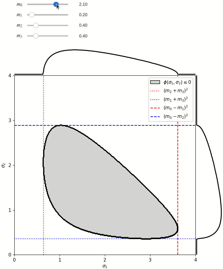
Kinematics for a three-body decay \(0 \to 123\) can be fully described by two Mandelstam variables \(\sigma_1, \sigma_2\), because the third variable \(\sigma_3\) can be expressed in terms \(\sigma_1, \sigma_2\), the mass \(m_0\) of the initial state, and the masses \(m_1, m_2, m_3\) of the final state. As can be seen, the roles of \(\sigma_1, \sigma_2, \sigma_3\) are interchangeable.

\[\displaystyle \sigma_{3} = m_{0}^{2} + m_{1}^{2} + m_{2}^{2} + m_{3}^{2} - \sigma_{1} - \sigma_{2}\]

The phase space is defined by the closed area that satisfies the condition \(\phi(\sigma_1,\sigma_2) \leq 0\), where \(\phi\) is a Kibble function:

\[\displaystyle \phi\left(\sigma_{1}, \sigma_{2}\right) = \lambda\left(\lambda\left(\sigma_{2}, m_{2}^{2}, m_{0}^{2}\right), \lambda\left(\sigma_{3}, m_{3}^{2}, m_{0}^{2}\right), \lambda\left(\sigma_{1}, m_{1}^{2}, m_{0}^{2}\right)\right)\]

and \(\lambda\) is the Källén function:

\[\displaystyle \lambda\left(x, y, z\right) = x^{2} - 2 x y - 2 x z + y^{2} - 2 y z + z^{2}\]

Any distribution over the phase space can now be defined using a two-dimensional grid over a Mandelstam pair \(\sigma_1,\sigma_2\) of choice, with the condition \(\phi(\sigma_1,\sigma_2)<0\) selecting the values that are physically allowed.

\[\begin{split}\displaystyle \begin{cases} 1 & \text{for}\: \phi\left(\sigma_{1}, \sigma_{2}\right) \leq 0 \\\text{NaN} & \text{otherwise} \end{cases}\end{split}\]

phsp_expr = is_within_phasespace(s1, s2, m0, m1, m2, m3, outside_value=0)
phsp_func = create_parametrized_function(
    phsp_expr.doit(),
    parameters={m0: 2.2, m1: 0.2, m2: 0.4, m3: 0.4},
    backend="numpy",
)

Show code cell source Hide code cell source

sliders = {
    "m0": FloatSlider(description="m0", max=3, value=2.1, step=0.01),
    "m1": FloatSlider(description="m1", max=2, value=0.2, step=0.01),
    "m2": FloatSlider(description="m2", max=2, value=0.4, step=0.01),
    "m3": FloatSlider(description="m3", max=2, value=0.4, step=0.01),
}

resolution = 300
X, Y = np.meshgrid(
    np.linspace(0, 4, num=resolution),
    np.linspace(0, 4, num=resolution),
)
data = {"sigma1": X, "sigma2": Y}

sidebar_ratio = 0.15
fig, ((ax1, _), (ax, ax2)) = plt.subplots(
    figsize=(7, 7),
    ncols=2,
    nrows=2,
    gridspec_kw={
        "height_ratios": [sidebar_ratio, 1],
        "width_ratios": [1, sidebar_ratio],
    },
)
_.remove()
ax.set_xlim(0, 4)
ax.set_ylim(0, 4)
ax.set_xlabel(R"$\sigma_1$")
ax.set_ylabel(R"$\sigma_2$")
ax.set_xticks(range(5))
ax.set_yticks(range(5))
ax1.set_xlim(0, 4)
ax2.set_ylim(0, 4)
for a in [ax1, ax2]:
    a.set_xticks([])
    a.set_yticks([])
    a.axis("off")
fig.tight_layout()
fig.subplots_adjust(wspace=0, hspace=0)

fig.canvas.toolbar_visible = False
fig.canvas.header_visible = False
fig.canvas.footer_visible = False

MESH: QuadContourSet | None = None
PROJECTIONS: tuple[Line2D, Line2D] = None
BOUNDARIES: list[Line2D] | None = None


def plot(**parameters):
    draw_boundaries(
        parameters["m0"],
        parameters["m1"],
        parameters["m2"],
        parameters["m3"],
    )
    global MESH, PROJECTIONS
    if MESH is not None:
        for coll in MESH.collections:
            ax.collections.remove(coll)
    phsp_func.update_parameters(parameters)
    Z = phsp_func(data)
    MESH = ax.contour(X, Y, Z, colors="black")
    contour = MESH.collections[0]
    contour.set_facecolor("lightgray")
    x = X[0]
    y = Y[:, 0]
    Zx = np.nansum(Z, axis=0)
    Zy = np.nansum(Z, axis=1)
    if PROJECTIONS is None:
        PROJECTIONS = (
            ax1.plot(x, Zx, c="black", lw=2)[0],
            ax2.plot(Zy, y, c="black", lw=2)[0],
        )
    else:
        PROJECTIONS[0].set_data(x, Zx)
        PROJECTIONS[1].set_data(Zy, y)
    ax1.relim()
    ax2.relim()
    ax1.autoscale_view(scalex=False)
    ax2.autoscale_view(scaley=False)
    create_legend(ax)
    fig.canvas.draw()


def draw_boundaries(m0, m1, m2, m3) -> None:
    global BOUNDARIES
    s1_min = (m2 + m3) ** 2
    s1_max = (m0 - m1) ** 2
    s2_min = (m1 + m3) ** 2
    s2_max = (m0 - m2) ** 2
    if BOUNDARIES is None:
        BOUNDARIES = [
            ax.axvline(s1_min, c="red", ls="dotted", label="$(m_2+m_3)^2$"),
            ax.axhline(s2_min, c="blue", ls="dotted", label="$(m_1+m_3)^2$"),
            ax.axvline(s1_max, c="red", ls="dashed", label="$(m_0-m_1)^2$"),
            ax.axhline(s2_max, c="blue", ls="dashed", label="$(m_0-m_2)^2$"),
        ]
    else:
        BOUNDARIES[0].set_data(get_line_data(s1_min))
        BOUNDARIES[1].set_data(get_line_data(s2_min, horizontal=True))
        BOUNDARIES[2].set_data(get_line_data(s1_max))
        BOUNDARIES[3].set_data(get_line_data(s2_max, horizontal=True))


def create_legend(ax: Axis):
    if ax.get_legend() is not None:
        return
    label = Rf"${sp.latex(kibble)}\leq0$"
    ax.legend(
        handles=[
            Patch(label=label, ec="black", fc="lightgray"),
            *BOUNDARIES,
        ],
        loc="upper right",
        facecolor="white",
        framealpha=1,
    )


def get_line_data(value, horizontal: bool = False) -> np.ndarray:
    pair = (value, value)
    if horizontal:
        return np.array([(0, 1), pair])
    return np.array([pair, (0, 1)])


output = interactive_output(plot, controls=sliders)
VBox([output, *sliders.values()])

The phase space boundary can be described analytically in terms of \(\sigma_1\) or \(\sigma_2\), in which case there are two solutions:

sol1, sol2 = sp.solve(kibble.doit().subs(s3, computed_s3), s2)

\[\begin{split}\displaystyle \begin{array}{c} \frac{- m_{0}^{2} m_{2}^{2} + m_{0}^{2} m_{3}^{2} + m_{0}^{2} \sigma_{1} + m_{1}^{2} m_{2}^{2} - m_{1}^{2} m_{3}^{2} + m_{1}^{2} \sigma_{1} + m_{2}^{2} \sigma_{1} + m_{3}^{2} \sigma_{1} - \sigma_{1}^{2} - \sqrt{\left(m_{0}^{2} - 2 m_{0} m_{1} + m_{1}^{2} - \sigma_{1}\right) \left(m_{0}^{2} + 2 m_{0} m_{1} + m_{1}^{2} - \sigma_{1}\right) \left(m_{2}^{2} - 2 m_{2} m_{3} + m_{3}^{2} - \sigma_{1}\right) \left(m_{2}^{2} + 2 m_{2} m_{3} + m_{3}^{2} - \sigma_{1}\right)}}{2 \sigma_{1}} \\ \frac{- m_{0}^{2} m_{2}^{2} + m_{0}^{2} m_{3}^{2} + m_{0}^{2} \sigma_{1} + m_{1}^{2} m_{2}^{2} - m_{1}^{2} m_{3}^{2} + m_{1}^{2} \sigma_{1} + m_{2}^{2} \sigma_{1} + m_{3}^{2} \sigma_{1} - \sigma_{1}^{2} + \sqrt{\left(m_{0}^{2} - 2 m_{0} m_{1} + m_{1}^{2} - \sigma_{1}\right) \left(m_{0}^{2} + 2 m_{0} m_{1} + m_{1}^{2} - \sigma_{1}\right) \left(m_{2}^{2} - 2 m_{2} m_{3} + m_{3}^{2} - \sigma_{1}\right) \left(m_{2}^{2} + 2 m_{2} m_{3} + m_{3}^{2} - \sigma_{1}\right)}}{2 \sigma_{1}} \\ \end{array}\end{split}\]

The boundary cannot be parametrized analytically in polar coordinates, but there is a numeric solution. The idea is to solve the condition \(\phi(\sigma_1,\sigma_2)=0\) after the following substitutions:

\[\begin{split}\displaystyle \begin{array}{rcl} \sigma_{1} &=& T_{1} + \left(m_{2} + m_{3}\right)^{2} \\ \sigma_{2} &=& T_{2} + \left(m_{1} + m_{3}\right)^{2} \\ \sigma_{3} &=& T_{3} + \left(m_{1} + m_{2}\right)^{2} \\ T_{1} &=& \frac{T_{0}}{3} - r \cos{\left(\theta \right)} \\ T_{2} &=& \frac{T_{0}}{3} + r \sin{\left(\theta + \frac{\pi}{6} \right)} \\ T_{3} &=& \frac{T_{0}}{3} + r \cos{\left(\theta + \frac{\pi}{3} \right)} \\ T_{0} &=& m_{0}^{2} + m_{1}^{2} + m_{2}^{2} + m_{3}^{2} - \left(m_{1} + m_{2}\right)^{2} - \left(m_{1} + m_{3}\right)^{2} - \left(m_{2} + m_{3}\right)^{2} \\ \end{array}\end{split}\]

For every value of \(\theta \in [0, 2\pi)\), the value of \(r\) can now be found by solving the condition \(\phi(r, \theta)=0\). Note that \(\phi(r, \theta)\) is a cubic polynomial of \(r\). For instance, if we take \(m_0=5, m_1=2, m_{2,3}=1\):

\[\begin{split}\displaystyle \begin{eqnarray} \phi(r, \theta) & = & r^{3} \cdot \left(56 \sqrt{3} \sin{\left(\theta \right)} + 400 \cos^{3}{\left(\theta \right)} - 356 \cos{\left(\theta \right)} + 112 \cos{\left(\theta + \frac{\pi}{3} \right)}\right) \nonumber\\ & & + r^{2} \cdot \left(2000 \cos^{2}{\left(\theta \right)} + 2100\right) \nonumber\\ & & - 4800 r \cos{\left(\theta \right)} \nonumber\\ & & + -25200 \end{eqnarray}\end{split}\]

The lowest value of \(r\) that satisfies \(\phi(r,\theta)=0\) defines the phase space boundary.