\Lambda_b^0 \to p K^- \gamma

$\Lambda_b^0 \to p K^- \gamma$#

We construct an amplitude model for the radiative decay studied by LHCb [3], using DalitzPlotDecompositionBuilder. The notebook makes the pK resonance content, LS couplings, dynamics, and numerical parameters explicit. It follows \Lambda_c^+ \to p \pi^+ K^- and uses the pinned reference model as the source of the values below.

The reference contains 13 $\Lambda^*$ resonances and a nonresonant $J^P=3/2^-$ contribution, with 74 production LS components in total. We retain their masses, widths, radii, and complex weights. The final plot illustrates this amplitude construction without detector acceptance, backgrounds, or the normalization of the experimental likelihood.

Decay definition#

Assign indices $1=p$, $2=K^-$, and $3=\gamma$, so all resonance dynamics depend on $\sigma_3=m^2(pK^-)$. The parent has spin $1/2$ and the photon has spin one and zero mass. Masses and widths are in GeV.

The resonance table lists $(J,P,m,\Gamma,l)$, where $l$ is the orbital angular momentum in $\Lambda^*\to pK^-$. For $\Lambda(1405)$, the zero width entry is unused because its two-channel denominator is defined below. The nonresonant entry has no pole. The reference labels the $\Lambda(1670)$ propagator L1680_BW; its mass parameter is $1.674\,\mathrm{GeV}$, which we retain.

name	LaTeX	$J^P$	mass (MeV)	width (MeV)
`L1405`	$\Lambda(1405)$	$\frac{1}{2}^-$	1,405	0
`L1520`	$\Lambda(1520)$	$\frac{3}{2}^-$	1,519	16
`L1600`	$\Lambda(1600)$	$\frac{1}{2}^+$	1,600	200
`L1670`	$\Lambda(1670)$	$\frac{1}{2}^-$	1,674	30
`L1690`	$\Lambda(1690)$	$\frac{3}{2}^-$	1,690	70
`L1800`	$\Lambda(1800)$	$\frac{1}{2}^-$	1,800	200
`L1810`	$\Lambda(1810)$	$\frac{1}{2}^+$	1,790	110
`L1820`	$\Lambda(1820)$	$\frac{5}{2}^+$	1,820	80
`L1830`	$\Lambda(1830)$	$\frac{5}{2}^-$	1,825	90
`L1890`	$\Lambda(1890)$	$\frac{3}{2}^+$	1,890	120
`L2100`	$\Lambda(2100)$	$\frac{7}{2}^-$	2,100	200
`L2110`	$\Lambda(2110)$	$\frac{5}{2}^+$	2,090	250
`L2350`	$\Lambda(2350)$	$\frac{9}{2}^+$	2,350	150
`LNR3O`	$\mathrm{NR}_{3/2^-}$	$\frac{3}{2}^-$	0	0

Production LS components#

At the weak radiative vertex, several $(L,S)$ combinations contribute to each resonance. At the strong vertex, the proton and kaon have total spin $1/2$ and the orbital angular momentum $l$ is fixed by the resonance spin and parity.

The following weights multiply the product of the production and decay LS recoupling factors. Each key is a resonance name and its production $(L,S)$; the decay indices are always $(l,1/2)$. They are copied from the reference model in its LS convention. This is why the vertex-factor normalization below must match that convention.

These 74 components are not independent fit parameters: the publication relates the highest-$S$ couplings to the others to account for the photon’s missing longitudinal state. We preserve the resulting reference weights and explicitly sum only over the two transverse photon helicities below.

Show the reference LS weights

Hide code cell source

ls_weights = {
    ("L1405", 0, "1/2"): 2.262 - 1.799j,
    ("L1405", 1, "1/2"): -1.872 - 1.044j,
    ("L1405", 1, "3/2"): 1.323 + 0.7382j,
    ("L1405", 2, "3/2"): -1.613 + 1.283j,
    ("L1520", 0, "1/2"): 4.108 - 0.06685j,
    ("L1520", 1, "1/2"): 5.529 + 0.8175j,
    ("L1520", 1, "3/2"): -1.67 + 21.2j,
    ("L1520", 2, "3/2"): -5.803 + 10.33j,
    ("L1520", 2, "5/2"): 5.024 - 3.492j,
    ("L1520", 3, "5/2"): 4.75 - 6.557j,
    ("L1600", 0, "1/2"): -4.985 - 7.276j,
    ("L1600", 1, "1/2"): 5.196 - 0.4418j,
    ("L1600", 1, "3/2"): -3.674 + 0.3124j,
    ("L1600", 2, "3/2"): 3.557 + 5.192j,
    ("L1670", 0, "1/2"): -0.1642 + 0.07875j,
    ("L1670", 1, "1/2"): 0.3371 + 0.2064j,
    ("L1670", 1, "3/2"): -0.2384 - 0.1459j,
    ("L1670", 2, "3/2"): 0.1172 - 0.0562j,
    ("L1690", 0, "1/2"): -1.252 - 0.2081j,
    ("L1690", 1, "1/2"): 6.391 + 5.315j,
    ("L1690", 1, "3/2"): 4.393 + 1.183j,
    ("L1690", 2, "3/2"): 8.022 + 6.075j,
    ("L1690", 2, "5/2"): -3.615 - 2.182j,
    ("L1690", 3, "5/2"): 3.352 + 3.624j,
    ("L1800", 0, "1/2"): 1.0 + 0.0j,
    ("L1800", 1, "1/2"): 0.3217 - 4.42j,
    ("L1800", 1, "3/2"): -0.2275 + 3.126j,
    ("L1800", 2, "3/2"): -0.7139 + 0.0j,
    ("L1810", 0, "1/2"): 1.233 + 0.5797j,
    ("L1810", 1, "1/2"): -0.1504 + 0.3181j,
    ("L1810", 1, "3/2"): 0.1064 - 0.2249j,
    ("L1810", 2, "3/2"): -0.8801 - 0.4138j,
    ("L1820", 1, "3/2"): 7.59 + 1.351j,
    ("L1820", 2, "3/2"): 12.7 + 33.14j,
    ("L1820", 2, "5/2"): 4.087 + 24.98j,
    ("L1820", 3, "5/2"): -9.183 + 32.97j,
    ("L1820", 3, "7/2"): 8.508 - 6.223j,
    ("L1820", 4, "7/2"): 9.944 + 22.67j,
    ("L1830", 1, "3/2"): -1.004 + 1.043j,
    ("L1830", 2, "3/2"): -1.846 - 0.7347j,
    ("L1830", 2, "5/2"): 1.614 + 1.209j,
    ("L1830", 3, "5/2"): -1.454 - 0.9561j,
    ("L1830", 3, "7/2"): -0.5284 + 1.101j,
    ("L1830", 4, "7/2"): -1.951 - 0.9064j,
    ("L1890", 0, "1/2"): -0.8057 + 1.595j,
    ("L1890", 1, "1/2"): -1.119 - 0.1973j,
    ("L1890", 1, "3/2"): 1.254 - 0.02961j,
    ("L1890", 2, "3/2"): -0.4407 - 3.386j,
    ("L1890", 2, "5/2"): -0.4595 + 2.329j,
    ("L1890", 3, "5/2"): -1.273 - 0.1395j,
    ("L2100", 2, "5/2"): 49.22 - 29.27j,
    ("L2100", 3, "5/2"): 51.79 + 112.5j,
    ("L2100", 3, "7/2"): 14.47 + 76.34j,
    ("L2100", 4, "7/2"): -59.3 + 160.7j,
    ("L2100", 4, "9/2"): 54.39 - 53.56j,
    ("L2100", 5, "9/2"): 44.59 + 88.99j,
    ("L2110", 1, "3/2"): 7.078 - 6.719j,
    ("L2110", 2, "3/2"): 20.67 + 20.61j,
    ("L2110", 2, "5/2"): 1.022 + 10.97j,
    ("L2110", 3, "5/2"): -0.804 + 32.73j,
    ("L2110", 3, "7/2"): 6.207 - 13.04j,
    ("L2110", 4, "7/2"): 17.51 + 15.18j,
    ("L2350", 3, "7/2"): 8.633 + 32.75j,
    ("L2350", 4, "7/2"): -26.5 + 36.77j,
    ("L2350", 4, "9/2"): -26.68 + 115.4j,
    ("L2350", 5, "9/2"): -56.26 + 16.55j,
    ("L2350", 5, "11/2"): 15.76 + 28.48j,
    ("L2350", 6, "11/2"): -21.37 + 18.42j,
    ("LNR3O", 0, "1/2"): 0.2015 + 0.1374j,
    ("LNR3O", 1, "1/2"): -0.9128 + 0.009663j,
    ("LNR3O", 1, "3/2"): 0.7796 - 0.00483j,
    ("LNR3O", 2, "3/2"): -0.324 - 0.1124j,
    ("LNR3O", 2, "5/2"): 0.1587 + 0.07209j,
    ("LNR3O", 3, "5/2"): -0.3178 + 0.002978j,
}

\[\displaystyle \Lambda_b^0\left[\frac{1}{2}^+\right] \xrightarrow[S=1/2]{L=0} \left(\Lambda(1520)\left[\frac{3}{2}^-\right] \xrightarrow[S=1/2]{L=2} p\left[\frac{1}{2}^+\right] K^-\left[0^-\right]\right) \gamma\left[1^-\right]\]

Lineshapes for dynamics#

The resonances other than $\Lambda(1405)$ use the unity-numerator running-width Breit–Wigner, $$ \mathcal R(s)=\frac{1}{m_R^2-s-i m_R\Gamma_R(s)}. $$

Both vertices carry Blatt–Weisskopf factors evaluated at the running pK mass, with $R_{\Lambda_b}=5$ and $R_\mathrm{res}=1.5$ in $\mathrm{GeV}^{-1}$. Their normalization is the unnormalized convention of the reference model, obtained by dividing AmpForm’s form factor by $|h_L^{(1)}(1)|$. The running width uses the ratio of the decay factors at $s$ and at the pole, so this constant cancels there.

For $\Lambda(1405)$, use $$ \mathcal R_{1405}(s)= \frac{1}{m_{1405}^2-s-i g^2\left[\rho_{pK}(s)+\rho_{\Sigma\pi}(s)\right]}, \qquad g^2=0.2494\,\mathrm{GeV}^2, $$

with $m_\Sigma = 1.197\,\mathrm{GeV}$ and $m_\pi = 0.14\,\mathrm{GeV}$. The phase-space factors are analytically continued below threshold.

The nonresonant term has a constant propagator and momentum factors $q_\mathrm{prod}^{L}q_\mathrm{dec}^{2}$ instead of Blatt–Weisskopf factors.

The builder returns each dynamics function as a named subexpression. This keeps the angular amplitudes readable and lets the numerical transformer evaluate each distinct dynamics function once per grid point.

\[\begin{split}\displaystyle \begin{aligned} \mathcal{R}^{\Lambda(1520)}_{0} \;&=\; \frac{\sqrt{13} \mathcal{R}^\mathrm{BW}_{L=2}\left(\sigma_{3}; m_{\Lambda(1520)}, \Gamma_{\Lambda(1520)}\right) \mathcal{F}_{0}\left(m_{0}^{2}, \sqrt{\sigma_{3}}, 0\right) \mathcal{F}_{2}\left(\sigma_{3}, m_{1}, m_{2}\right)}{13} \\ \end{aligned}\end{split}\]

Model formulation#

Select LS couplings at both vertices and use one complex coefficient per LS chain. The coefficient symbol carries the resonance name, followed by the production $(L,S)$ and decay $(l,1/2)$ indices. Assigning the weights after formulation keeps the parameters available for later variation.

Subsystem 3 is the natural alignment frame because every chain has a pK isobar. The general builder sums over all spin-one projections. A real photon has only $\lambda_\gamma=\pm1$, so we explicitly restrict the outer intensity sum to these two helicities. No rotation of the photon to a different subsystem is required in this model.

The reference convention includes an explicit $\sqrt{2J_R+1}$ multiplying each chain amplitude. The general builder uses the same normalized LS recoupling factors but leaves this factor in the coefficient. We therefore assign $c_\mathrm{builder}=\sqrt{2J_R+1}\,c_\mathrm{reference}$.

builder = DalitzPlotDecompositionBuilder(decay, min_ls=False)
for resonance in resonances.values():
    builder.dynamics_choices.register_builder(resonance.name, formulate_dynamics)
model = builder.formulate(reference_subsystem=3, use_coefficients=True)
assigned_coefficients = set()
for (name, orbital, spin), weight in ls_weights.items():
    resonance = resonances[name]
    decay_orbital = resonance_parameters[name][4]
    coefficient = sp.IndexedBase(Rf"\mathcal{{H}}^\mathrm{{LS,{resonance.latex}}}")[
        orbital, sp.Rational(spin), decay_orbital, sp.Rational(1, 2)
    ]
    assert coefficient in model.parameter_defaults
    model.parameter_defaults[coefficient] = (
        np.sqrt(float(2 * resonance.spin + 1)) * weight
    )
    assigned_coefficients.add(coefficient)
assert len(assigned_coefficients) == len(chains)
photon_helicity = sp.Symbol("lambda3", rational=True)
model = evolve(
    model,
    intensity=PoolSum(
        model.intensity.expression,
        *(
            (symbol, (-1, 1) if symbol == photon_helicity else values)
            for symbol, values in model.intensity.indices
        ),
    ),
)
model.intensity

\[\displaystyle \sum_{\lambda_{0}=-1/2}^{1/2} \sum_{\lambda_{1}=-1/2}^{1/2} \sum_{\lambda_{2}=0} \sum_{\lambda_{3}\in\left\{-1,1\right\}}{\left|{\sum_{\lambda_0^{\prime}=-1/2}^{1/2} \sum_{\lambda_1^{\prime}=-1/2}^{1/2} \sum_{\lambda_2^{\prime}=0} \sum_{\lambda_3^{\prime}=-1}^{1}{A^{3}_{\lambda_0^{\prime}, \lambda_1^{\prime}, \lambda_2^{\prime}, \lambda_3^{\prime}} d^{\frac{1}{2}}_{\lambda_1^{\prime},\lambda_{1}}\left(\zeta^1_{3(3)}\right) d^{\frac{1}{2}}_{\lambda_{0},\lambda_0^{\prime}}\left(\zeta^0_{3(3)}\right) d^{1}_{\lambda_3^{\prime},\lambda_{3}}\left(\zeta^3_{3(3)}\right)}}\right|^{2}}\]

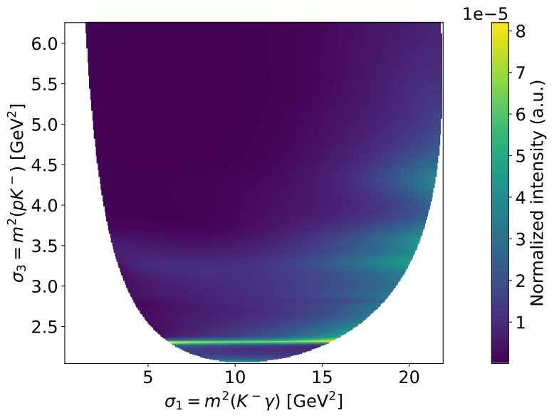
The model now contains the reference LS weights and dynamics, with a transverse photon in the intensity sum. This is an explicit DPD reconstruction. Comparisons of absolute intensities with another implementation also require matching helicity sums, alignment conventions, and normalization; the Dalitz plot below is normalized independently.

Numerical evaluation#

Substitute the numerical defaults and transform the invariant masses to the helicity angles required by the amplitudes. The third invariant follows from $\sigma_1+\sigma_2+\sigma_3=m_{\Lambda_b}^2+m_p^2+m_K^2$.

Dalitz plot#

The axes are $\sigma_1=m^2(K^-\gamma)$ and $\sigma_3=m^2(pK^-)$. We restrict $m(pK^-)$ to $2.5\,\mathrm{GeV}$, the upper limit of the published analysis [3], and evaluate only the physical interior. This resolves the narrow $\Lambda(1520)$ band while keeping the model within the studied mass range. The resonance bands illustrate the pK dynamics and their coherent interference; this plot includes neither detector efficiency nor event selection.

_images/e88ef8534fd70b5f7b6955197ce6124f6c06087d85cc12884758c6e5918ebaef.svg

\Lambda_b^0 \to p K^- \gamma

Contents

\(\Lambda_b^0 \to p K^- \gamma\)#