


\(X \to \pi^-\pi^+\pi^-\)#

This notebook constructs a Dalitz-plot decomposition for the \(\rho(770)\pi\) P-wave in the COMPASS three-pion analysis [4]. We define the particles, the two pion pairings, their LS couplings, and the running-width dynamics explicitly, following the model-building approach of \Lambda_c^+ \to p \pi^+ K^-.

The numerical inputs come from the pinned amplitude-serialization model. We reconstruct its selected spin-one wave at \(m_X=1.55\,\mathrm{GeV}\), rather than the full production analysis. The fitted coefficient sets the wave’s overall scale; the two identical negative pions require coherent contributions from both \(\pi^+\pi^-\) pairings.

Decay definition#

The final-state indices are \(1=\pi^-\), \(2=\pi^+\), and \(3=\pi^-\). Both vertices have orbital angular momentum \(L=1\): \(X\to\rho\pi\) couples the daughter spins to \(S=1\), while \(\rho\to\pi\pi\) has \(S=0\). All masses and widths below are in GeV.

Hide code cell source

states = {
    0: State("X", "X", spin=1, parity=-1, mass=1.55, width=0, index=0),
    1: State("pi-", R"\pi^-", spin=0, parity=-1, mass=0.1396, width=0, index=1),
    2: State("pi+", R"\pi^+", spin=0, parity=-1, mass=0.1396, width=0, index=2),
    3: State("pi-", R"\pi^-", spin=0, parity=-1, mass=0.1396, width=0, index=3),
}
rho = Particle("rho(770)", R"\rho(770)", spin=1, parity=-1, mass=0.7685, width=0.1507)
chains = [
    ThreeBodyDecayChain(
        IsobarNode(
            states[0],
            IsobarNode(rho, states[i], states[j], interaction=(1, 0)),
            states[k],
            interaction=(1, 1),
        )
    )
    for i, j, k in [(2, 3, 1), (1, 2, 3)]
]
decay = ThreeBodyDecay(states, chains)
Markdown(as_markdown_table([states[0], rho, states[1], states[2]]))

index

name

LaTeX

\(J^P\)

mass (MeV)

width (MeV)

0

X

\(X\)

\(1^-\)

1,550

0

rho(770)

\(\rho(770)\)

\(1^-\)

768

150

1

pi-

\(\pi^-\)

\(0^-\)

139

0

2

pi+

\(\pi^+\)

\(0^-\)

139

0

Hide code cell source

Math(aslatex(decay, with_jp=True))
\[\begin{split}\displaystyle \begin{array}{c} X\left[1^-\right] \xrightarrow[S=1]{L=1} \left(\rho(770)\left[1^-\right] \xrightarrow[S=0]{L=1} \pi^+\left[0^-\right] \pi^-\left[0^-\right]\right) \pi^-\left[0^-\right] \\ X\left[1^-\right] \xrightarrow[S=1]{L=1} \left(\rho(770)\left[1^-\right] \xrightarrow[S=0]{L=1} \pi^-\left[0^-\right] \pi^+\left[0^-\right]\right) \pi^-\left[0^-\right] \\ \end{array}\end{split}\]

Lineshapes for dynamics#

For each \(\rho\) contribution, use

\[ \mathcal R(s)=\frac{F_1(m_X^2;\sqrt{s},m_\pi,R_X)\,F_1(s;m_\pi,m_\pi,R_\rho)} {m_\rho^2-s-i m_\rho\Gamma_\rho(s)},\qquad \Gamma_\rho(s)=\Gamma_\rho\left(\frac{q(s)}{q(m_\rho^2)}\right)^3 \frac{1+q^2(m_\rho^2)R_\rho^2}{1+q^2(s)R_\rho^2}. \]

This running width follows the reference expression, which has no additional \(m_\rho/\sqrt{s}\) factor. The vertex factors use the unnormalized Blatt–Weisskopf convention: AmpForm’s \(L=1\) form factor is divided by \(\sqrt{2}\). The radii are \(R_X=4.941\) and \(R_\rho=4.94\) in \(\mathrm{GeV}^{-1}\).

The DPD cyclic ordering makes the P-wave amplitudes antisymmetric under exchange of the negative pions. An explicit relative minus sign between the two chains produces a symmetric total amplitude. We put that sign in the dynamics builder so that the two pairings can share one coefficient.

Hide code cell source

def formulate_rho_dynamics(chain: ThreeBodyDecayChain) -> DefinedExpression:
    s = get_mandelstam_s(chain.decay_node)
    m_parent, m_pion, m_rho, width, r_parent, r_rho = sp.symbols(
        "m0 m_pi m_rho Gamma_rho R_X R_rho", nonnegative=True
    )
    q_squared = BreakupMomentumSquared(s, m_pion, m_pion)
    q0_squared = BreakupMomentumSquared(m_rho**2, m_pion, m_pion)
    running_width = (
        width
        * (q_squared / q0_squared) ** sp.Rational(3, 2)
        * (1 + q0_squared * r_rho**2)
        / (1 + q_squared * r_rho**2)
    )
    production = FormFactor(m_parent**2, sp.sqrt(s), m_pion, 1, r_parent) / sp.sqrt(2)
    decay_factor = FormFactor(s, m_pion, m_pion, 1, r_rho) / sp.sqrt(2)
    sign = 1 if chain.spectator.index == 1 else -1
    return DefinedExpression(
        sign
        * production
        * decay_factor
        / (m_rho**2 - s - sp.I * m_rho * running_width),
        {
            m_parent: chain.parent.mass,
            m_pion: chain.decay_products[0].mass,
            m_rho: chain.resonance.mass,
            width: chain.resonance.width,
            r_parent: 4.941,
            r_rho: 4.94,
        },
    )

Hide code cell source

Math(aslatex(formulate_rho_dynamics(chains[0]).expression))
\[\displaystyle \frac{\mathcal{F}_{1}\left(m_{0}^{2}, \sqrt{\sigma_{1}}, m_{\pi}\right) \mathcal{F}_{1}\left(\sigma_{1}, m_{\pi}, m_{\pi}\right)}{2 \left(- \frac{i \Gamma_{\rho} m_{\rho} \left(\frac{q^2_{1}\left(\sigma_{1}\right)}{q^2\left(m_{\rho}^{2}\right)}\right)^{\frac{3}{2}} \left(R_{\rho}^{2} q^2\left(m_{\rho}^{2}\right) + 1\right)}{R_{\rho}^{2} q^2_{1}\left(\sigma_{1}\right) + 1} + m_{\rho}^{2} - \sigma_{1}\right)}\]

Model formulation#

Select LS couplings at both vertices with min_ls=False and combine their product into a single complex coefficient with use_coefficients=True. The coefficient indices are \((L_\mathrm{prod},S_\mathrm{prod},L_\mathrm{dec},S_\mathrm{dec})\). Both pairings have the same coefficient; their relative sign is already in the dynamics.

The reference convention includes an explicit \(\sqrt{2J_R+1}\) multiplying each chain amplitude. The general builder uses the same normalized LS recoupling factors but leaves this factor in the coefficient. We therefore assign \(c_\mathrm{builder}=\sqrt{2J_R+1}\,c_\mathrm{reference}\).

builder = DalitzPlotDecompositionBuilder(decay, min_ls=False)
builder.dynamics_choices.register_builder(chains[0], formulate_rho_dynamics)
model = builder.formulate(reference_subsystem=1, use_coefficients=True)
coefficient = sp.IndexedBase(R"\mathcal{H}^\mathrm{LS,\rho(770)}")[1, 1, 1, 0]
assert coefficient in model.parameter_defaults
reference_weight = -0.003616 + 0.0418j
model.parameter_defaults[coefficient] = (
    np.sqrt(float(2 * rho.spin + 1)) * reference_weight
)
model.intensity
\[\displaystyle \sum_{\lambda_{0}=-1}^{1} \sum_{\lambda_{1}=0} \sum_{\lambda_{2}=0} \sum_{\lambda_{3}=0}{\left|{\sum_{\lambda_0^{\prime}=-1}^{1} \sum_{\lambda_1^{\prime}=0} \sum_{\lambda_2^{\prime}=0} \sum_{\lambda_3^{\prime}=0}{A^{1}_{\lambda_0^{\prime}, \lambda_1^{\prime}, \lambda_2^{\prime}, \lambda_3^{\prime}} d^{1}_{\lambda_{0},\lambda_0^{\prime}}\left(\zeta^0_{1(1)}\right) + A^{3}_{\lambda_0^{\prime}, \lambda_1^{\prime}, \lambda_2^{\prime}, \lambda_3^{\prime}} d^{1}_{\lambda_{0},\lambda_0^{\prime}}\left(\zeta^0_{3(1)}\right)}}\right|^{2}}\]

Hide code cell source

Math(aslatex(model.amplitudes, terms_per_line=1))
\[\begin{split}\displaystyle \begin{aligned} A^{1}_{-1, 0, 0, 0} \;&=\; \sum_{\lambda_{R}=-1}^{1}{\frac{\delta_{-1 \lambda_{R}} C^{0,0}_{0,0,0,0} C^{1,0}_{1,0,0,0} C^{1,\lambda_{R}}_{1,0,1,\lambda_{R}} C^{1,\lambda_{R}}_{1,\lambda_{R},0,0} \mathcal{F}_{1}\left(m_{0}^{2}, \sqrt{\sigma_{1}}, m_{\pi}\right) \mathcal{F}_{1}\left(\sigma_{1}, m_{\pi}, m_{\pi}\right) \mathcal{H}^\mathrm{LS,\rho(770)}_{1, 1, 1, 0} d^{1}_{\lambda_{R},0}\left(\theta_{23}\right)}{2 \left(- \frac{i \Gamma_{\rho} m_{\rho} \left(\frac{q^2_{1}\left(\sigma_{1}\right)}{q^2\left(m_{\rho}^{2}\right)}\right)^{\frac{3}{2}} \left(R_{\rho}^{2} q^2\left(m_{\rho}^{2}\right) + 1\right)}{R_{\rho}^{2} q^2_{1}\left(\sigma_{1}\right) + 1} + m_{\rho}^{2} - \sigma_{1}\right)}} \\ A^{3}_{-1, 0, 0, 0} \;&=\; \sum_{\lambda_{R}=-1}^{1}{- \frac{\delta_{-1 \lambda_{R}} C^{0,0}_{0,0,0,0} C^{1,0}_{1,0,0,0} C^{1,\lambda_{R}}_{1,0,1,\lambda_{R}} C^{1,\lambda_{R}}_{1,\lambda_{R},0,0} \mathcal{F}_{1}\left(m_{0}^{2}, \sqrt{\sigma_{3}}, m_{\pi}\right) \mathcal{F}_{1}\left(\sigma_{3}, m_{\pi}, m_{\pi}\right) \mathcal{H}^\mathrm{LS,\rho(770)}_{1, 1, 1, 0} d^{1}_{\lambda_{R},0}\left(\theta_{12}\right)}{2 \left(- \frac{i \Gamma_{\rho} m_{\rho} \left(\frac{q^2_{3}\left(\sigma_{3}\right)}{q^2\left(m_{\rho}^{2}\right)}\right)^{\frac{3}{2}} \left(R_{\rho}^{2} q^2\left(m_{\rho}^{2}\right) + 1\right)}{R_{\rho}^{2} q^2_{3}\left(\sigma_{3}\right) + 1} + m_{\rho}^{2} - \sigma_{3}\right)}} \\ A^{1}_{0, 0, 0, 0} \;&=\; \sum_{\lambda_{R}=-1}^{1}{\frac{\delta_{0 \lambda_{R}} C^{0,0}_{0,0,0,0} C^{1,0}_{1,0,0,0} C^{1,\lambda_{R}}_{1,0,1,\lambda_{R}} C^{1,\lambda_{R}}_{1,\lambda_{R},0,0} \mathcal{F}_{1}\left(m_{0}^{2}, \sqrt{\sigma_{1}}, m_{\pi}\right) \mathcal{F}_{1}\left(\sigma_{1}, m_{\pi}, m_{\pi}\right) \mathcal{H}^\mathrm{LS,\rho(770)}_{1, 1, 1, 0} d^{1}_{\lambda_{R},0}\left(\theta_{23}\right)}{2 \left(- \frac{i \Gamma_{\rho} m_{\rho} \left(\frac{q^2_{1}\left(\sigma_{1}\right)}{q^2\left(m_{\rho}^{2}\right)}\right)^{\frac{3}{2}} \left(R_{\rho}^{2} q^2\left(m_{\rho}^{2}\right) + 1\right)}{R_{\rho}^{2} q^2_{1}\left(\sigma_{1}\right) + 1} + m_{\rho}^{2} - \sigma_{1}\right)}} \\ A^{3}_{0, 0, 0, 0} \;&=\; \sum_{\lambda_{R}=-1}^{1}{- \frac{\delta_{0 \lambda_{R}} C^{0,0}_{0,0,0,0} C^{1,0}_{1,0,0,0} C^{1,\lambda_{R}}_{1,0,1,\lambda_{R}} C^{1,\lambda_{R}}_{1,\lambda_{R},0,0} \mathcal{F}_{1}\left(m_{0}^{2}, \sqrt{\sigma_{3}}, m_{\pi}\right) \mathcal{F}_{1}\left(\sigma_{3}, m_{\pi}, m_{\pi}\right) \mathcal{H}^\mathrm{LS,\rho(770)}_{1, 1, 1, 0} d^{1}_{\lambda_{R},0}\left(\theta_{12}\right)}{2 \left(- \frac{i \Gamma_{\rho} m_{\rho} \left(\frac{q^2_{3}\left(\sigma_{3}\right)}{q^2\left(m_{\rho}^{2}\right)}\right)^{\frac{3}{2}} \left(R_{\rho}^{2} q^2\left(m_{\rho}^{2}\right) + 1\right)}{R_{\rho}^{2} q^2_{3}\left(\sigma_{3}\right) + 1} + m_{\rho}^{2} - \sigma_{3}\right)}} \\ A^{1}_{1, 0, 0, 0} \;&=\; \sum_{\lambda_{R}=-1}^{1}{\frac{\delta_{1 \lambda_{R}} C^{0,0}_{0,0,0,0} C^{1,0}_{1,0,0,0} C^{1,\lambda_{R}}_{1,0,1,\lambda_{R}} C^{1,\lambda_{R}}_{1,\lambda_{R},0,0} \mathcal{F}_{1}\left(m_{0}^{2}, \sqrt{\sigma_{1}}, m_{\pi}\right) \mathcal{F}_{1}\left(\sigma_{1}, m_{\pi}, m_{\pi}\right) \mathcal{H}^\mathrm{LS,\rho(770)}_{1, 1, 1, 0} d^{1}_{\lambda_{R},0}\left(\theta_{23}\right)}{2 \left(- \frac{i \Gamma_{\rho} m_{\rho} \left(\frac{q^2_{1}\left(\sigma_{1}\right)}{q^2\left(m_{\rho}^{2}\right)}\right)^{\frac{3}{2}} \left(R_{\rho}^{2} q^2\left(m_{\rho}^{2}\right) + 1\right)}{R_{\rho}^{2} q^2_{1}\left(\sigma_{1}\right) + 1} + m_{\rho}^{2} - \sigma_{1}\right)}} \\ A^{3}_{1, 0, 0, 0} \;&=\; \sum_{\lambda_{R}=-1}^{1}{- \frac{\delta_{1 \lambda_{R}} C^{0,0}_{0,0,0,0} C^{1,0}_{1,0,0,0} C^{1,\lambda_{R}}_{1,0,1,\lambda_{R}} C^{1,\lambda_{R}}_{1,\lambda_{R},0,0} \mathcal{F}_{1}\left(m_{0}^{2}, \sqrt{\sigma_{3}}, m_{\pi}\right) \mathcal{F}_{1}\left(\sigma_{3}, m_{\pi}, m_{\pi}\right) \mathcal{H}^\mathrm{LS,\rho(770)}_{1, 1, 1, 0} d^{1}_{\lambda_{R},0}\left(\theta_{12}\right)}{2 \left(- \frac{i \Gamma_{\rho} m_{\rho} \left(\frac{q^2_{3}\left(\sigma_{3}\right)}{q^2\left(m_{\rho}^{2}\right)}\right)^{\frac{3}{2}} \left(R_{\rho}^{2} q^2\left(m_{\rho}^{2}\right) + 1\right)}{R_{\rho}^{2} q^2_{3}\left(\sigma_{3}\right) + 1} + m_{\rho}^{2} - \sigma_{3}\right)}} \\ \end{aligned}\end{split}\]

Numerical evaluation#

The model contains helicity-angle expressions in model.variables. A TensorWaves transformer evaluates those angles from two independent Mandelstam invariants. Substituting the parameter defaults then gives a numerical intensity, without using the serialization compiler.

Hide code cell source

sigma1, sigma2, sigma3 = sp.symbols("sigma1:4", nonnegative=True)
definitions = dict(model.variables)
definitions[sigma2] = model.invariants[sigma2]
definitions = {
    symbol: expression.xreplace(definitions).xreplace(model.masses)
    for symbol, expression in definitions.items()
}
transformer = SympyDataTransformer.from_sympy(definitions, backend="numpy")
intensity_expression = cached.xreplace(cached.unfold(model), model.parameter_defaults)
intensity_function = cached.lambdify(intensity_expression, backend="numpy")

Dalitz plot#

Evaluate only points inside the physical Dalitz boundary. The plot uses \(\sigma_1=m^2(\pi^+_2\pi^-_3)\) and \(\sigma_3=m^2(\pi^-_1\pi^+_2)\). Exchanging the negative pions transposes these axes, so the intensity must be symmetric.
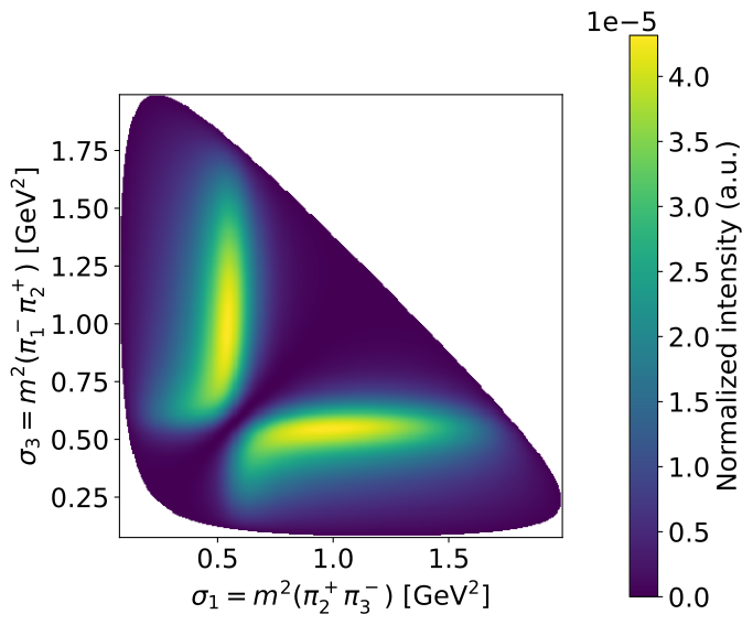
Hide code cell source

parent_mass = decay.initial_state.mass
m1, m2, m3 = (decay.final_state[i].mass for i in (1, 2, 3))
x = np.linspace((m2 + m3) ** 2, (parent_mass - m1) ** 2, 401)
y = np.linspace((m1 + m2) ** 2, (parent_mass - m3) ** 2, 401)
X, Y = np.meshgrid(x, y)
# the Kibble function is symmetric under relabeling (sigma2, m2) <-> (sigma3, m3)
phsp_indicator = is_within_phasespace(sigma1, sigma3, parent_mass, m1, m3, m2)
physical = np.isfinite(sp.lambdify((sigma1, sigma3), phsp_indicator.doit())(X, Y))
data = {"sigma1": X[physical], "sigma3": Y[physical]}
data.update(transformer(data))
intensities = np.full(X.shape, np.nan)
intensities[physical] = intensity_function(data)
assert np.all(np.isfinite(intensities[physical]))
assert np.all(intensities[physical] >= 0)
assert np.nanmax(intensities) > 0

Hide code cell source

exchanged = {"sigma1": data["sigma3"], "sigma3": data["sigma1"]}
exchanged.update(transformer(exchanged))
np.testing.assert_allclose(
    intensities[physical], intensity_function(exchanged), rtol=1e-10, atol=1e-12
)

Hide code cell source

plt.rc("font", size=18)
fig, ax = plt.subplots(figsize=(7, 6), constrained_layout=True)
mesh = ax.pcolormesh(X, Y, intensities / np.nansum(intensities), rasterized=True)
ax.set_aspect("equal")
ax.set_xlabel(R"$\sigma_1 = m^2(\pi^+_2\pi^-_3)$ [GeV$^2$]")
ax.set_ylabel(R"$\sigma_3 = m^2(\pi^-_1\pi^+_2)$ [GeV$^2$]")
fig.colorbar(mesh, ax=ax, label="Normalized intensity (a.u.)")
plt.show()
_images/0bafcdeff1ccd8b35a54c2f845669eec032ec738514b19725cae941002d9125d.svg