Data module¶

Warning

The pycompwa is no longer maintained. Use the ComPWA packages QRules, AmpForm, and TensorWaves instead!

The pycompwa.data module provides several tools for importing, exporting, and visualizing data. By data, we mean event-wise collections of four-momentum tuples, possibly organized by particle name. We choose to work with pandas as a back-end, because it allows fast manipulation and visualization of data sets and can import and export to several standard data formats.

This notebook shows how to conveniently manipulate momentum tuple collections in such a way that they can be imported into ComPWA. It is also shown how to import data from other frameworks and how to do conversions to kinematic variables.

PWA data frame¶

Input data for PWA frameworks mainly consists of event-wise four-momentum tuples, grouped by particle. The core of the data module is therefore handled by a specially formatted pandas.DataFrame. Such as specific format not only allows us to import and export to different file formats, but also to convert the data to ComPWA objects, such as an EventCollection.

The format is guaranteed through a decorator called register_dataframe_accessor(). Such an accessor extends a DataFrame with several properties, granted that the DataFrame properly validates according to that accessor. In the data module, this accessor is the PwaAccessor. We call a DataFrame that is formatted according to this accessor a PWA DataFrame.

To be sure, all this sounds a bit abstract. To illustrate the usage of this accessor, we therefore first have to create a skeleton PWA DataFrame. This can be done through the create module.

from pycompwa.data import create

2021-10-27 10:25:30,046 INFO [default] Logging to file disabled!
2021-10-27 10:25:30,046 [INFO] Log level: INFO
2021-10-27 10:25:30,046 [INFO] Current date and time: Wed Oct 27 10:25:30 2021

frame = create.pwa_frame(
    particle_names=["gamma", "pi0", "pi0"], number_of_rows=3
)
frame

Particle	gamma				pi0-1				pi0-2
Momentum	p_x	p_y	p_z	E	p_x	p_y	p_z	E	p_x	p_y	p_z	E
0	NaN	NaN	NaN	NaN	NaN	NaN	NaN	NaN	NaN	NaN	NaN	NaN
1	NaN	NaN	NaN	NaN	NaN	NaN	NaN	NaN	NaN	NaN	NaN	NaN
2	NaN	NaN	NaN	NaN	NaN	NaN	NaN	NaN	NaN	NaN	NaN	NaN

Note that his DataFrame has hierarchical column name (see multi-indexing): the first column layer is the particle name, the second contains the four-momentum labels. In addition, duplicate particle names have been made unique by adding an index. Values are undefined by default, but you can set them later on. Here, we do this manually, but you can use this procedure for importing large data sets in your own Python scripts.

frame["gamma", "p_x"] = [-0.520903, -0.285015, 0.632325]
frame["gamma", "p_y"] = [0.885259, 0.520381, -0.779928]
frame["gamma", "p_z"] = [0.655934, -0.996574, -0.892786]
frame["gamma", "E"] = [1.21872, 1.15982, 1.34357]

frame["pi0-1", "p_x"] = [0.653672, 0.452265, 0.113717]
frame["pi0-1", "p_y"] = [-0.813022, -0.76188, 0.605441]
frame["pi0-1", "p_z"] = [-1.01763, 0.00723327, 0.718613]
frame["pi0-1", "E"] = [1.46359, 0.896256, 0.956093]

frame["pi0-2", "p_x"] = [-0.132769, -0.16725, -0.746043]
frame["pi0-2", "p_y"] = [-0.0722372, 0.241499, 0.174487]
frame["pi0-2", "p_z"] = [0.361697, 0.989341, 0.174172]
frame["pi0-2", "E"] = [0.414596, 1.04082, 0.797233]

We can now already have a glance at some of the properties that the PwaAccessor offers. You can access these properties through the pwa namespace and perform some standard pandas computation on them:

print("Particles:", frame.pwa.particles)
print("Momentum labels:", frame.pwa.momentum_labels)
print("Weights:", frame.pwa.weights)
print("Average pi0 mass:\n", frame[["pi0-1", "pi0-2"]].pwa.mass.stack().mean())
print(
    "Average gamma 3-momentum:\n",
    frame["gamma"].pwa.rho.mean(),
    "+/-",
    frame["gamma"].pwa.rho.std(),
)

Particles: ['gamma', 'pi0-1', 'pi0-2']
Momentum labels: ['p_x', 'p_y', 'p_z', 'E']
Weights: None
Average pi0 mass:
 0.1349838859840143
Average gamma 3-momentum:
 1.2407047361464343 +/- 0.09382756371243478

We’ll see more of these properties after we import some real data.

Import and export data¶

The module data.io allows one to import from and to data formats of other PWA frameworks. Here’s an example, importing a pawianHists.root file. Such a file not only contains ROOT histograms of the kinematic distributions, but also two TTrees of four-momentum tuples: one for data and one for fit intensities.

from pycompwa.data import io

frame_data = io.pawian.read_hists_file("jpsi_f0_gammapipi.root", "data")
frame_fit = io.pawian.read_hists_file("jpsi_f0_gammapipi.root", "fit")
frame_fit

Particle	gamma				pi0_1				pi0_2				weight
Momentum	p_x	p_y	p_z	E	p_x	p_y	p_z	E	p_x	p_y	p_z	E
0	0.053254	-0.102226	-0.271504	0.294959	1.305630	-0.324557	0.223228	1.370420	-1.358880	0.426783	0.048276	1.43152	0.003513
1	-0.233270	0.509333	0.499320	0.750437	-0.684387	-0.801269	0.281889	1.099140	0.917657	0.291936	-0.781209	1.24733	0.008061
2	-0.300303	0.284337	-0.255063	0.485887	-1.020240	-0.026281	0.630984	1.207460	1.320550	-0.258056	-0.375920	1.40356	0.003586
3	0.555215	0.086553	0.825067	0.998244	-0.757501	0.411259	0.234126	0.903313	0.202285	-0.497813	-1.059190	1.19534	0.025217
4	0.649631	0.057455	-0.008806	0.652226	-0.923858	0.799518	-0.581799	1.359950	0.274227	-0.856973	0.590605	1.08473	0.004200
...	...	...	...	...	...	...	...	...	...	...	...	...	...
1505	-0.469609	-0.065891	-0.356168	0.593068	-0.845740	-0.168722	-0.402724	0.961326	1.315350	0.234614	0.758892	1.54251	0.004934
1506	0.680510	0.304596	-0.181785	0.767410	-0.805672	0.780103	-0.233644	1.153460	0.125162	-1.084700	0.415429	1.17603	0.006227
1507	-0.095390	0.716417	-1.176800	1.381018	0.061994	0.059014	-0.119087	0.199315	0.033396	-0.775431	1.295890	1.51656	19.929375
1508	-1.161710	-0.184147	0.105635	1.180948	-0.040109	-0.486701	-0.161686	0.531834	1.201820	0.670847	0.056052	1.38411	0.052588
1509	-0.062611	-0.288004	-0.153473	0.332296	0.192284	-0.350495	1.339660	1.404540	-0.129673	0.638500	-1.186190	1.36006	0.002482

1510 rows × 13 columns

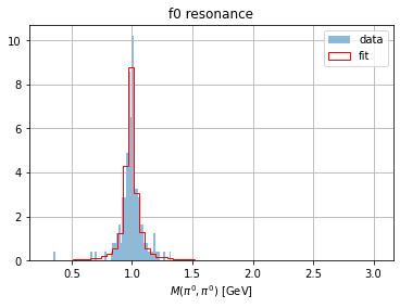
Note how, here too, the DataFrame is formatted in such a way that it can be handled by the PwaAccessor. Also note that the DataFrame for the fit result contains weights. As discussed in Step 4: Analyze results, these are the fit intensities for each data point in the phase space. This allows us to already make some quick visualization of invariant mass distribution of the resonance:

import matplotlib.pyplot as plt

f0_data = frame_data["pi0_1"] + frame_data["pi0_2"]
f0_fit = frame_fit["pi0_1"] + frame_fit["pi0_2"]

f0_data.pwa.mass.hist(label="data", bins=60, density=True, alpha=0.5)
f0_fit.pwa.mass.hist(
    label="fit",
    bins=60,
    density=True,
    histtype="step",
    color="red",
    weights=frame_fit.pwa.intensities,
)

plt.xlabel("$M(\pi^0,\pi^0)$ [GeV]")
plt.legend()
plt.gca().set_title("f0 resonance")
plt.show()

You can also easily export the data again after you’ve made some adjustments, like selecting certain events. Just to illustrate the benefits of pandas, we apply some filter on one of the \(\pi^0\) mass, export the frame to an ASCII file and import it again:

selection = frame_data[abs(f0_data.pwa.mass - 0.990) < 0.05]
io.pawian.write_ascii(selection, "filtered_data.dat")
io.pawian.read_ascii("filtered_data.dat", ["gamma", "pi0", "pi0"])

Particle	gamma				pi0-1				pi0-2
Momentum	p_x	p_y	p_z	E	p_x	p_y	p_z	E	p_x	p_y	p_z	E
0	-0.182506	-0.844948	1.076130	1.380327	0.141731	0.873233	-1.220080	1.513090	0.040775	-0.028285	0.143952	0.203479
1	0.559665	-0.873999	-0.921926	1.388181	0.030816	0.642806	0.822141	1.052750	-0.590482	0.231193	0.099785	0.655968
2	-1.030480	0.892277	0.264144	1.388459	0.681217	-1.064850	-0.251640	1.295960	0.349266	0.172571	-0.012504	0.412483
3	0.116316	1.265080	-0.564446	1.390164	0.132802	0.100997	0.095432	0.234868	-0.249118	-1.366070	0.469014	1.471870
4	-1.072190	-0.141766	0.861404	1.382645	1.230490	0.096587	-0.605567	1.381430	-0.158292	0.045179	-0.255837	0.332819
...	...	...	...	...	...	...	...	...	...	...	...	...
89	1.285130	0.549771	0.048662	1.398633	-0.325851	-0.492884	0.288127	0.671081	-0.959282	-0.056887	-0.336789	1.027180
90	0.351707	0.223883	-1.309260	1.374039	-0.370255	0.172147	1.221450	1.294940	0.018548	-0.396030	0.087812	0.427918
91	1.303890	0.441621	-0.203768	1.391646	-1.148060	-0.246995	0.510475	1.287580	-0.155831	-0.194626	-0.306707	0.417672
92	-0.524492	-0.265778	1.252710	1.383840	0.215780	-0.239497	-0.992715	1.052440	0.308712	0.505275	-0.259997	0.660624
93	0.545379	1.241510	0.242481	1.377528	0.198947	-0.082614	-0.218520	0.335223	-0.744326	-1.158900	-0.023961	1.384150

94 rows × 12 columns

Conversion to kinematic variables¶

Having a PWA DataFrame, we can use ComPWA to convert the momentum tuples to kinematic variables. For that, of course, we first need to create a model file for the kinematics. As can be seen from the column names of the PWA DataFrame that we imported from the pawianHists.root file, we have momentum tuples for a \(J/\psi \to \gamma\pi^0\pi^0\) decay and we saw that there is only one resonance (\(f_0(980)\)):

import logging

import pycompwa.ui as pwa

# not interested in warnings now
logger = logging.getLogger()
logger.setLevel(logging.ERROR)
pwa.Logging("ERROR");

2021-10-27 10:25:31,290 [INFO] Logging to file disabled!

from pycompwa.expertsystem.ui.system_control import (
    InteractionTypes,
    StateTransitionManager,
)

initial_state = [("J/psi", [-1, 1])]
final_state = [("gamma"), ("pi0"), ("pi0")]
tbd_manager = StateTransitionManager(
    initial_state,
    final_state,
    formalism_type="helicity",
    topology_building="isobar",
)

tbd_manager.set_allowed_interaction_types([InteractionTypes.EM])
tbd_manager.allowed_intermediate_particles = ["f0(980)"]

graph_interaction_settings_groups = tbd_manager.prepare_graphs()
solutions, _ = tbd_manager.find_solutions(graph_interaction_settings_groups)

from pycompwa.expertsystem.amplitude.helicitydecay import (
    HelicityAmplitudeGeneratorXML,
)

model_file = "jpsi_f0_gammapipi.xml"
xml_generator = HelicityAmplitudeGeneratorXML()
xml_generator.generate(solutions)
xml_generator.write_to_file(model_file)

Now that we have an XML model file defining the kinematics and a PWA DataFrame, we can use the convert module to convert the DataFrame to an EventCollection. Note, however, that we will run into an exception:

from pycompwa.data import convert

try:
    convert.pandas_to_events(frame_data, model_file)
except Exception as exc:
    print("EXCEPTION:", exc)

EXCEPTION: 
  You first have to convert the columns names:
    ['gamma', 'pi0_1', 'pi0_2']
  to the final state IDs:
    [2, 3, 4]
  as defined in XML file
    "jpsi_f0_gammapipi.xml"
  with e.g. naming.particle_to_id or pandas.DataFrame.rename

What’s going on here? The kinematics file works with final state IDs, so it doesn’t understand the particle names here. Now, we could try to follow the first suggestion here, but this won’t work:

from pycompwa.data import naming

naming.particle_to_id(frame_data, model_file)
frame_data.pwa.particles

[2, 'pi0_1', 'pi0_2']

As you can see, the \(\gamma\) has been nicely renamed to its final state ID, but the renaming failed for the pions (it would have worked if the separator used for the added index for duplicate particles were a -). If we follow the second suggestion, it will work:

mapping = {"gamma": 2, "pi0_1": 3, "pi0_2": 4}
frame_data.rename(columns=mapping, inplace=True)
frame_fit.rename(columns=mapping, inplace=True)
events_data = convert.pandas_to_events(frame_data, model_file)
events_fit = convert.pandas_to_events(frame_fit, model_file)

Now that you have EventCollection instances, you are free to use all ComPWA functionality from Step 3: Perform fit onwards. If, however, you were more interested in the kinematic variables for these imported data sets immediately, you can expand the original PWA DataFrame with the kinematic variables as follows:

import pycompwa.ui as pwa
from pycompwa.data import append

set_data = pwa.compute_kinematic_variables(events_data, model_file)
set_fit = pwa.compute_kinematic_variables(events_fit, model_file)
naming.id_to_particle(frame_data, model_file, make_unique=True)
naming.id_to_particle(frame_fit, model_file, make_unique=True)
append(frame_data, convert.data_set_to_pandas(set_data))
append(frame_fit, convert.data_set_to_pandas(set_fit))
frame_data.pwa.other_columns

['phi_2_34',
 'phi_24_3',
 'mSq_(2,3)',
 'phi_2_3_vs_4',
 'theta_2_34',
 'mSq_(2,4)',
 'theta_23_4',
 'mSq_(3,4)',
 'theta_24_3',
 'phi_2_4_vs_3',
 'phi_3_4_vs_2',
 'theta_2_3_vs_4',
 'phi_23_4',
 'theta_2_4_vs_3',
 'mSq_(2,3,4)',
 'theta_3_4_vs_2']

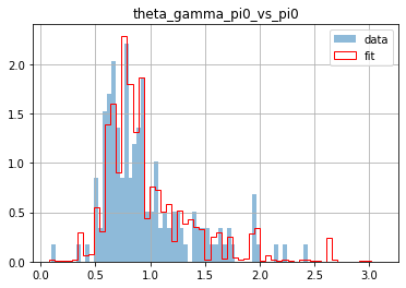
Finally, we can plot the distributions of the kinematic variables (as computed by ComPWA) of the imported data.

var = "theta_2_4_vs_3"
frame_data[var].hist(label="data", bins=60, density=True, alpha=0.5)
frame_fit[var].hist(
    label="fit",
    bins=60,
    density=True,
    histtype="step",
    color="red",
    weights=frame_fit.pwa.intensities,
)
plt.gca().set_title(naming.replace_ids(var, model_file))
plt.legend();