Step 4: Analyze results
Warning
The pycompwa is no longer maintained. Use the ComPWA packages QRules, AmpForm, and TensorWaves instead!
Note
We load the output from the previous steps first. Note that you need to define an estimator before loading the fit result to the intensity.
import pycompwa.ui as pwa
2021-10-27 10:28:00,481 INFO [default] Logging to file disabled!
2021-10-27 10:28:00,481 [INFO] Log level: INFO
2021-10-27 10:28:00,481 [INFO] Current date and time: Wed Oct 27 10:28:00 2021
pwa.Logging("error")  # at this stage, we are not interested in the back-end
particle_list = pwa.read_particles("model.xml")
kinematics = pwa.create_helicity_kinematics("model.xml", particle_list)
kinematics.create_all_subsystems()
data_sample = pwa.read_root_data(input_file="generated_data.root")
phsp_sample = pwa.read_root_data(input_file="generated_phsp.root")
intensity_builder = pwa.IntensityBuilderXML(
    "model.xml", particle_list, kinematics, phsp_sample
)
fit_result = pwa.load("fit_result.xml")
intensity = intensity_builder.create_intensity()
data_set = kinematics.convert(data_sample)
phsp_set = kinematics.convert(phsp_sample)
(
    estimator,
    initial_parameters,
) = pwa.create_unbinned_log_likelihood_function_tree_estimator(
    intensity, data_set
)
intensity.updateParametersFrom(fit_result.final_parameters)
2021-10-27 10:28:00,888 [INFO] Logging to file disabled!
4.1 Convert to pandas
It is easiest to analyze your data with pandas.DataFrame. We are mostly interested in the distributions of the kinematic variables, so we first have to convert the DataSet instances to a DataFrame. We can do this with the data.convert module:
from pycompwa.data import convert
frame_data = convert.data_set_to_pandas(data_set)
frame_phsp = convert.data_set_to_pandas(phsp_set)
frame_data
| phi_2_34 | phi_24_3 | mSq_(2,3) | phi_2_3_vs_4 | theta_2_34 | mSq_(2,4) | theta_23_4 | mSq_(3,4) | theta_34_2 | mSq_(2,3,4) | theta_3_4_vs_2 | phi_34_2 | phi_23_4 | theta_2_3_vs_4 | theta_24_3 | phi_2_4_vs_3 | phi_3_4_vs_2 | theta_2_4_vs_3 | |
|---|---|---|---|---|---|---|---|---|---|---|---|---|---|---|---|---|---|---|
| 0 | 2.102657 | 2.247974 | 7.041085 | 1.782934 | 1.002477 | 0.543847 | 2.745762 | 2.042295 | 2.139116 | 9.59079 | 0.502226 | -1.038936 | 0.498287 | 2.224991 | 0.797810 | -0.554556 | 0.463670 | 0.915063 |
| 1 | 2.071876 | 2.106510 | 3.162373 | 0.072829 | 2.604591 | 4.057776 | 2.852961 | 2.407078 | 0.537001 | 9.59079 | 1.697711 | -1.069717 | -0.965088 | 1.299054 | 1.578960 | -0.020714 | 0.040498 | 1.424155 |
| 2 | -0.889536 | -1.756459 | 4.671107 | -0.724954 | 2.297602 | 3.687157 | 1.794325 | 1.268963 | 0.843991 | 9.59079 | 1.448707 | 2.252057 | -0.229754 | 1.039627 | 2.432907 | 1.456694 | -2.095938 | 0.938116 |
| 3 | 2.007197 | -3.122791 | 2.253370 | 1.288726 | 1.385250 | 3.558244 | 0.925994 | 3.815613 | 1.756343 | 9.59079 | 1.800957 | -1.134396 | 1.112438 | 1.595627 | 2.159360 | -1.965977 | 2.245262 | 1.827414 |
| 4 | -2.553175 | -3.092292 | 1.277894 | -0.255728 | 1.157882 | 5.765827 | 0.701375 | 2.583506 | 1.983710 | 9.59079 | 2.277980 | 0.588417 | -2.428574 | 1.152534 | 2.789166 | 2.649058 | -2.962439 | 1.918852 |
| ... | ... | ... | ... | ... | ... | ... | ... | ... | ... | ... | ... | ... | ... | ... | ... | ... | ... | ... |
| 9995 | -0.222349 | 0.534366 | 3.694790 | 0.860415 | 2.257719 | 1.919805 | 1.999034 | 4.012632 | 0.883873 | 9.59079 | 1.243871 | 2.919244 | -2.017723 | 1.929566 | 1.716018 | -0.771193 | 1.101634 | 1.600783 |
| 9996 | -1.343847 | -1.411040 | 6.871474 | -0.685393 | 0.886257 | 0.165163 | 2.657135 | 2.590590 | 2.255336 | 9.59079 | 0.238120 | 1.797745 | 1.425939 | 2.746994 | 0.773063 | 0.435808 | -0.390363 | 0.879317 |
| 9997 | -1.598526 | -0.592358 | 2.555019 | 1.917279 | 0.627246 | 6.196502 | 0.665568 | 0.875706 | 2.514347 | 9.59079 | 2.022378 | 1.543067 | -2.206541 | 0.684207 | 1.084305 | -2.424707 | 1.715182 | 1.026751 |
| 9998 | -2.735183 | 0.200863 | 0.232193 | 0.320457 | 1.459895 | 5.701769 | 1.247911 | 3.693265 | 1.681698 | 9.59079 | 2.783947 | 0.406410 | -2.805244 | 1.244396 | 2.221093 | -0.384746 | 2.836304 | 2.694432 |
| 9999 | -2.831066 | 2.733274 | 4.462864 | -1.123583 | 2.271190 | 4.105117 | 2.130626 | 1.059246 | 0.870403 | 9.59079 | 1.527329 | 0.310527 | -2.036393 | 0.914699 | 2.111935 | 1.100360 | -1.532029 | 0.881110 |
10000 rows × 18 columns
We converted the phase space sample as well, because it serves as a uniform space over which to evaluate the intensity model. We therefore attribute an intensity as a weight to each entry in the phase space DataFrame:
intensity_set = intensity.evaluate(phsp_set.data)
frame_phsp["weights"] = intensity_set
Hint
The pycompwa.data contains several tools for converting from and to pandas.DataFrame. There is also a data.io submodule, which allows you to import form and export to file formats of other PWA frameworks. A demonstration of this module can be found under Data module.
4.2 Visualize
Now that we converted our data to pandas.DataFrame, we can use its full potential! In this section, we will use some of that DataFrame functionality to create histograms of the distributions of the kinematic variables and will have a look at the Dalitz plots both data and fit result.
Kinematic variables
Currently, the columns of the DataFrame created above contain final state IDs. Of course, you would rather see particle names there, but we need to use unique IDs in case there are identical particle names. The data.naming module provides a tool that can convert the final state IDs to recognizable names:
from pycompwa.data import naming

naming.replace_ids("2,3", "model.xml")
'gamma,pi0'
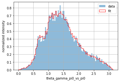
Now you can apply the usual matplotlib.pyplot tools to plot the distributions.
import matplotlib.pyplot as plt
def plot_1d_comparison(name, bins=100, **kwargs):
    """Helper function for comparing the 1D distributions of fit and data."""
    frame_data[name].hist(
        bins=bins, density=True, alpha=0.5, label="data", **kwargs
    )
    frame_phsp[name].hist(
        bins=bins,
        weights=frame_phsp["weights"],
        density=True,
        histtype="step",
        color="red",
        label="fit",
        **kwargs,
    )
    plt.ylabel("normalized intensity")
    title = naming.replace_ids(name, kinematics)
    plt.xlabel(title)
plot_1d_comparison("theta_2_4_vs_3")
plt.legend();
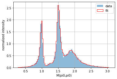
Applying a transformation to one of the columns is also easily done for a pandas.DataFrame. For instance, if you are interested in the invariant mass (and not the square value of the invariant mass), simply use numpy.sqrt():
from numpy import sqrt

frame_data["M(3,4)"] = sqrt(frame_data["mSq_(3,4)"])
frame_phsp["M(3,4)"] = sqrt(frame_phsp["mSq_(3,4)"])

plot_1d_comparison("M(3,4)")
plt.legend();
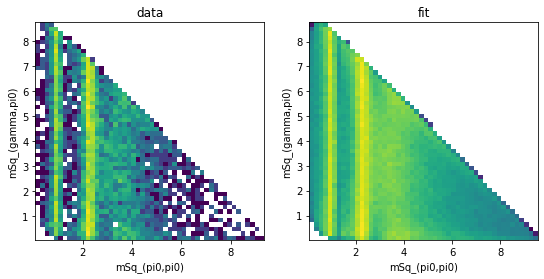
Dalitz plots
Dalitz plots are 2-dimensional histograms of the square values of the invariant masses. We are therefore interested in the following variables:
variable_names = data_set.data.keys()
[var for var in variable_names if var.startswith("mSq_")]
['mSq_(2,3)', 'mSq_(2,4)', 'mSq_(3,4)', 'mSq_(2,3,4)']
We now use hist2d() to generate the Dalitz plots:
def dalitz_plot(frame, mass_x, mass_y, bins=50, **kwargs):
    """Helper function to create a Dalitz plot with useful axis titles."""
    plt.hist2d(frame[mass_x], frame[mass_y], bins=bins, **kwargs)
    plt.xlabel(naming.replace_ids(mass_x, kinematics))
    plt.ylabel(naming.replace_ids(mass_y, kinematics))
from matplotlib.colors import LogNorm  # logarithmic z-axis

fig, axs = plt.subplots(1, 2, figsize=(9, 4))

plt.sca(axs[0])
axs[0].set_title("data")
dalitz_plot(frame_data, "mSq_(3,4)", "mSq_(2,4)", norm=LogNorm())

plt.sca(axs[1])
axs[1].set_title("fit")
dalitz_plot(
    frame_phsp,
    "mSq_(3,4)",
    "mSq_(2,4)",
    norm=LogNorm(),
    weights=frame_phsp["weights"],
)
4.3 Calculate fit fractions
The original intensity model that we optimized consists of several components. All registered component names can be retrieved via get_all_component_names():
intensity_builder.get_all_component_names()
{'J/psi_-1_to_f0(1500)_0+gamma_-1;f0(1500)_0_to_pi0_0+pi0_0;': 'Amplitude',
 'J/psi_-1_to_f0(1500)_0+gamma_1;f0(1500)_0_to_pi0_0+pi0_0;': 'Amplitude',
 'J/psi_-1_to_f0(980)_0+gamma_-1;f0(980)_0_to_pi0_0+pi0_0;': 'Amplitude',
 'J/psi_-1_to_f0(980)_0+gamma_1;f0(980)_0_to_pi0_0+pi0_0;': 'Amplitude',
 'J/psi_-1_to_f2(1270)_-1+gamma_-1;f2(1270)_-1_to_pi0_0+pi0_0;': 'Amplitude',
 'J/psi_-1_to_f2(1270)_-2+gamma_-1;f2(1270)_-2_to_pi0_0+pi0_0;': 'Amplitude',
 'J/psi_-1_to_f2(1270)_0+gamma_-1;f2(1270)_0_to_pi0_0+pi0_0;': 'Amplitude',
 'J/psi_-1_to_f2(1270)_0+gamma_1;f2(1270)_0_to_pi0_0+pi0_0;': 'Amplitude',
 'J/psi_-1_to_f2(1270)_1+gamma_1;f2(1270)_1_to_pi0_0+pi0_0;': 'Amplitude',
 'J/psi_-1_to_f2(1270)_2+gamma_1;f2(1270)_2_to_pi0_0+pi0_0;': 'Amplitude',
 'J/psi_-1_to_f2(1950)_-1+gamma_-1;f2(1950)_-1_to_pi0_0+pi0_0;': 'Amplitude',
 'J/psi_-1_to_f2(1950)_-2+gamma_-1;f2(1950)_-2_to_pi0_0+pi0_0;': 'Amplitude',
 'J/psi_-1_to_f2(1950)_0+gamma_-1;f2(1950)_0_to_pi0_0+pi0_0;': 'Amplitude',
 'J/psi_-1_to_f2(1950)_0+gamma_1;f2(1950)_0_to_pi0_0+pi0_0;': 'Amplitude',
 'J/psi_-1_to_f2(1950)_1+gamma_1;f2(1950)_1_to_pi0_0+pi0_0;': 'Amplitude',
 'J/psi_-1_to_f2(1950)_2+gamma_1;f2(1950)_2_to_pi0_0+pi0_0;': 'Amplitude',
 'J/psi_1_to_f0(1500)_0+gamma_-1;f0(1500)_0_to_pi0_0+pi0_0;': 'Amplitude',
 'J/psi_1_to_f0(1500)_0+gamma_1;f0(1500)_0_to_pi0_0+pi0_0;': 'Amplitude',
 'J/psi_1_to_f0(980)_0+gamma_-1;f0(980)_0_to_pi0_0+pi0_0;': 'Amplitude',
 'J/psi_1_to_f0(980)_0+gamma_1;f0(980)_0_to_pi0_0+pi0_0;': 'Amplitude',
 'J/psi_1_to_f2(1270)_-1+gamma_-1;f2(1270)_-1_to_pi0_0+pi0_0;': 'Amplitude',
 'J/psi_1_to_f2(1270)_-2+gamma_-1;f2(1270)_-2_to_pi0_0+pi0_0;': 'Amplitude',
 'J/psi_1_to_f2(1270)_0+gamma_-1;f2(1270)_0_to_pi0_0+pi0_0;': 'Amplitude',
 'J/psi_1_to_f2(1270)_0+gamma_1;f2(1270)_0_to_pi0_0+pi0_0;': 'Amplitude',
 'J/psi_1_to_f2(1270)_1+gamma_1;f2(1270)_1_to_pi0_0+pi0_0;': 'Amplitude',
 'J/psi_1_to_f2(1270)_2+gamma_1;f2(1270)_2_to_pi0_0+pi0_0;': 'Amplitude',
 'J/psi_1_to_f2(1950)_-1+gamma_-1;f2(1950)_-1_to_pi0_0+pi0_0;': 'Amplitude',
 'J/psi_1_to_f2(1950)_-2+gamma_-1;f2(1950)_-2_to_pi0_0+pi0_0;': 'Amplitude',
 'J/psi_1_to_f2(1950)_0+gamma_-1;f2(1950)_0_to_pi0_0+pi0_0;': 'Amplitude',
 'J/psi_1_to_f2(1950)_0+gamma_1;f2(1950)_0_to_pi0_0+pi0_0;': 'Amplitude',
 'J/psi_1_to_f2(1950)_1+gamma_1;f2(1950)_1_to_pi0_0+pi0_0;': 'Amplitude',
 'J/psi_1_to_f2(1950)_2+gamma_1;f2(1950)_2_to_pi0_0+pi0_0;': 'Amplitude',
 'coherent_J/psi_-1_to_gamma_-1+pi0_0+pi0_0': 'Intensity',
 'coherent_J/psi_-1_to_gamma_1+pi0_0+pi0_0': 'Intensity',
 'coherent_J/psi_1_to_gamma_-1+pi0_0+pi0_0': 'Intensity',
 'coherent_J/psi_1_to_gamma_1+pi0_0+pi0_0': 'Intensity',
 'incoherent_with_strength': 'Intensity'}
As you can see, these components are amplitudes and intensities that are added coherently or incoherently.
In PWA, you are often interested in the fractions that those amplitudes contribute to the total intensity. These fit fractions can be calculated using the fit_fractions_with_propagated_errors() function. It requires amplitude or Intensity components that can be extracted from the IntensityBuilderXML instance. A nested list of the component names has to be specified as well. These are the names specified in the component XML attributes. If the inner lists contain more than one component, these components will be added coherently. In this way, you can calculate your own customized fit fractions.
components = intensity_builder.create_intensity_components(
    [
        ["coherent_J/psi_-1_to_gamma_-1+pi0_0+pi0_0"],
        ["J/psi_-1_to_f2(1270)_-1+gamma_-1;f2(1270)_-1_to_pi0_0+pi0_0;"],
        ["J/psi_-1_to_f2(1270)_-2+gamma_-1;f2(1270)_-2_to_pi0_0+pi0_0;"],
        ["J/psi_-1_to_f2(1270)_0+gamma_-1;f2(1270)_0_to_pi0_0+pi0_0;"],
        [
            "J/psi_-1_to_f2(1270)_-1+gamma_-1;f2(1270)_-1_to_pi0_0+pi0_0;",
            "J/psi_-1_to_f2(1270)_-2+gamma_-1;f2(1270)_-2_to_pi0_0+pi0_0;",
            "J/psi_-1_to_f2(1270)_0+gamma_-1;f2(1270)_0_to_pi0_0+pi0_0;",
        ],
    ]
)
The last step is to call the actual fit fraction calculation function fit_fractions_with_propagated_errors(). Here, the first required argument is a list of component pairs. Each pair resembles the nominator and denominator of a fit fraction.
fit_fractions = pwa.fit_fractions_with_propagated_errors(
    [
        (components[1], components[0]),
        (components[2], components[0]),
        (components[3], components[0]),
        (components[4], components[0]),
    ],
    phsp_set,
    fit_result,
)
for fraction in fit_fractions:
    print(fraction.name.replace(";", "\n  "))
    print(fraction.value, "+/-", fraction.error)
    print()
J/psi_-1_to_f2(1270)_-1+gamma_-1
  f2(1270)_-1_to_pi0_0+pi0_0
  /coherent_J/psi_-1_to_gamma_-1+pi0_0+pi0_0
0.005501850830271934 +/- 0.0022183924278350166

J/psi_-1_to_f2(1270)_-2+gamma_-1
  f2(1270)_-2_to_pi0_0+pi0_0
  /coherent_J/psi_-1_to_gamma_-1+pi0_0+pi0_0
0.012420672414339593 +/- 0.0026534378040259095

J/psi_-1_to_f2(1270)_0+gamma_-1
  f2(1270)_0_to_pi0_0+pi0_0
  /coherent_J/psi_-1_to_gamma_-1+pi0_0+pi0_0
0.010391539894976263 +/- 0.002190682079425624

J/psi_-1_to_f2(1270)_-1+gamma_-1
  f2(1270)_-1_to_pi0_0+pi0_0
  _J/psi_-1_to_f2(1270)_-2+gamma_-1
  f2(1270)_-2_to_pi0_0+pi0_0
  _J/psi_-1_to_f2(1270)_0+gamma_-1
  f2(1270)_0_to_pi0_0+pi0_0
  /coherent_J/psi_-1_to_gamma_-1+pi0_0+pi0_0
0.028241292333928133 +/- 0.0029959295033270307
That’s it! You can check some of the other examples to learn about more detailed features of ComPWA.
And, please, feel free to provide feedback or contribute ;)