Lecture 2 – Kinematics

Lecture 2 by Vincent Mathieu contains a few data files containing four-momenta data samples. Our goal in this notebook is to identify which reaction was used to generate these data samples.

Three-particles-1.dat

Import Python libraries

Hide code cell content

import warnings

import gdown
import numpy as np
from IPython.display import display

warnings.filterwarnings("ignore")

filename = gdown.cached_download(
    url="https://indico.ific.uv.es/event/6803/contributions/21220/attachments/11209/15504/Three-particles-1.dat",
    path="data/Three-particles-1.dat",
    md5="a49ebfd97ae6a02023291df665ab924c",
    quiet=True,
    verify=False,
)
data = np.loadtxt(filename)
data.shape

(400000, 4)

n_final_state = 3
pa, p1, p2, p3 = (data[i::4].T for i in range(n_final_state + 1))
p0 = p1 + p2 + p3
pb = p0 - pa

def mass(p: np.ndarray) -> np.ndarray:
    return np.sqrt(mass_squared(p))


def mass_squared(p: np.ndarray) -> np.ndarray:
    return p[0] ** 2 - np.sum(p[1:] ** 2, axis=0)


m0 = mass(p0)
print(f"{m0.mean():.4g} +/- {m0.std():.4g}")

4.102 +/- 4.992e-07

Show code cell source

Hide code cell source

from IPython.display import Math

display(Math(Rf"m_a = {mass(pa).mean():.3g}\text{{ GeV}}"))
display(Math(Rf"m_b = {mass(pb).mean():.3g}\text{{ GeV}}"))
for i, p in enumerate([p0, p1, p2, p3]):
    display(Math(Rf"m_{i} = {mass(p).mean():.3g}\text{{ GeV}}"))

\[\displaystyle m_a = 0\text{ GeV}\]

\[\displaystyle m_b = 0.938\text{ GeV}\]

\[\displaystyle m_0 = 4.1\text{ GeV}\]

\[\displaystyle m_1 = 0.548\text{ GeV}\]

\[\displaystyle m_2 = 0.135\text{ GeV}\]

\[\displaystyle m_3 = 0.938\text{ GeV}\]

Identify final state particles

Hide code cell source

from particle import Particle


def find_candidates(
    mass: float, delta: float = 0.001, charge: float | None = None
) -> list[Particle]:
    def identify(p) -> bool:
        if p.pdgid == 21:
            return None
        if charge is not None and p.charge != charge:
            return False
        return mass - delta < 0.001 * p.mass < mass + delta

    return Particle.findall(identify)


ma = mass(pa).mean()
mb = mass(pb).mean()
m1 = mass(p1).mean()
m2 = mass(p2).mean()
m3 = mass(p3).mean()
initial_state = (
    find_candidates(ma.mean(), delta=1e-4)[0],
    find_candidates(mb.mean())[0],
)
final_state = tuple(find_candidates(m.mean())[0] for m in [m1, m2, m3])
display(
    Math(R"\text{Incoming: }" + ", ".join(f"{p.latex_name}" for p in initial_state)),
    Math(R"\text{Outgoing: }" + ", ".join(f"{p.latex_name}" for p in final_state)),
)

\[\displaystyle \text{Incoming: }\gamma, p\]

\[\displaystyle \text{Outgoing: }\eta, \pi^{0}, p\]

So this is a photon \(\gamma\) hitting a proton \(p\) and producing a meson \(\eta\), pion \(\pi^0\), and proton \(p\).

Dalitz plot

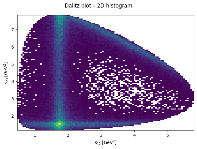
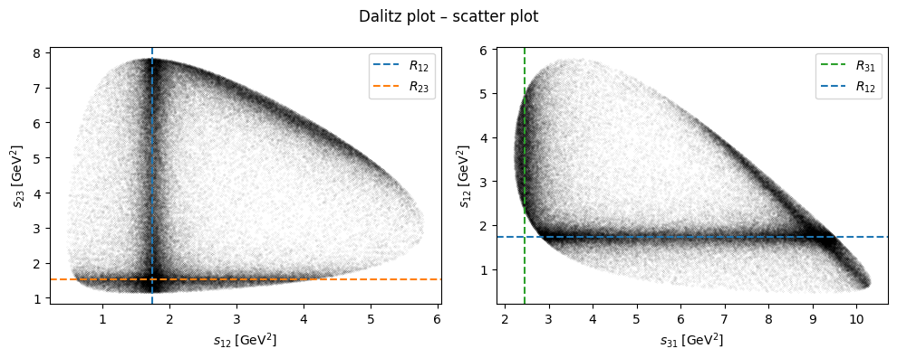
By plotting the three Mandelstam variables in a Dalitz plot, we can identify resonances appear in the reaction for which this data was generated.

s12 = mass_squared(p1 + p2)
s23 = mass_squared(p2 + p3)
s31 = mass_squared(p3 + p1)

m12 = mass(p1 + p2)
m23 = mass(p2 + p3)
m31 = mass(p3 + p1)

Show code cell source

Hide code cell source

import matplotlib.pyplot as plt

fig, ax = plt.subplots()
fig.suptitle("Dalitz plot – 2D histogram")
ax.hist2d(s12, s23, bins=100, cmin=1)
ax.set_xlabel(R"$s_{12}\;\left[\mathrm{GeV}^2\right]$")
ax.set_ylabel(R"$s_{23}\;\left[\mathrm{GeV}^2\right]$")
fig.tight_layout()
plt.show()

R12 = 1.74
R23 = 1.53
R31 = 2.45

Show code cell source

Hide code cell source

fig, (ax1, ax2) = plt.subplots(figsize=(10, 4), ncols=2)
fig.suptitle("Dalitz plot – scatter plot")
ax1.scatter(s12, s23, c="black", s=1e-3)
ax1.set_xlabel(R"$s_{12}\;\left[\mathrm{GeV}^2\right]$")
ax1.set_ylabel(R"$s_{23}\;\left[\mathrm{GeV}^2\right]$")
ax1.axvline(R12, c="C0", ls="dashed", label="$R_{12}$")
ax1.axhline(R23, c="C1", ls="dashed", label="$R_{23}$")
ax1.legend()
ax2.scatter(s31, s12, c="black", s=1e-3)
ax2.set_xlabel(R"$s_{31}\;\left[\mathrm{GeV}^2\right]$")
ax2.set_ylabel(R"$s_{12}\;\left[\mathrm{GeV}^2\right]$")
ax2.axvline(R31, c="C2", ls="dashed", label="$R_{31}$")
ax2.axhline(R12, c="C0", ls="dashed", label="$R_{12}$")
ax2.legend()
fig.tight_layout()
plt.show()

Particle identification

In the following, we make a few cuts on Mandelstam variables to select a region where the resonances lie isolated. We then use these cuts as a filter on the computed masses for each each and then compute the mean.

m12_mean = m12[(s12 < 3) & (s23 > 2.5) & (s23 < 10)].mean()
m12_mean**2

np.float64(1.7290722578143247)

m23_mean = m23[s23 < 2.5].mean()
m23_mean**2

np.float64(1.6561439882106896)

m31_mean = m31[(s12 > 3) & (s31 < 4)].mean()
m31_mean**2

np.float64(2.692708758538996)

The particle candidates for \(R_{12} \to \eta\pi^0\), \(R_{23} \to \pi^0 p\), and \(R_{31} \to p\eta\) are then:

find_candidates(mass=np.sqrt(R12), delta=0.01, charge=0)

[<Particle: name="a(2)(1320)0", pdgid=115, mass=1318.2 ± 0.6 MeV>,
 <Particle: name="Xi0", pdgid=3322, mass=1314.86 ± 0.20 MeV>,
 <Particle: name="Xi~0", pdgid=-3322, mass=1314.86 ± 0.20 MeV>]

find_candidates(mass=np.sqrt(R23), delta=0.01, charge=+1)

[<Particle: name="Delta(1232)~+", pdgid=-1114, mass=1232.0 ± 2.0 MeV>,
 <Particle: name="Delta(1232)+", pdgid=2214, mass=1232.0 ± 2.0 MeV>,
 <Particle: name="b(1)(1235)+", pdgid=10213, mass=1230 ± 3 MeV>,
 <Particle: name="a(1)(1260)+", pdgid=20213, mass=1230 ± 40 MeV>]

find_candidates(mass=np.sqrt(R31), delta=0.01, charge=+1)

[<Particle: name="Delta(1600)~+", pdgid=-31114, mass=1570 ± 70 MeV>,
 <Particle: name="Delta(1600)+", pdgid=32214, mass=1570 ± 70 MeV>]

Three-particles-2.dat

Load data

Hide code cell content

filename2 = gdown.cached_download(
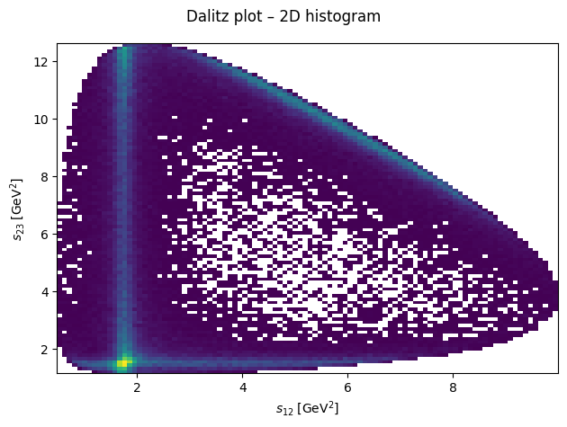
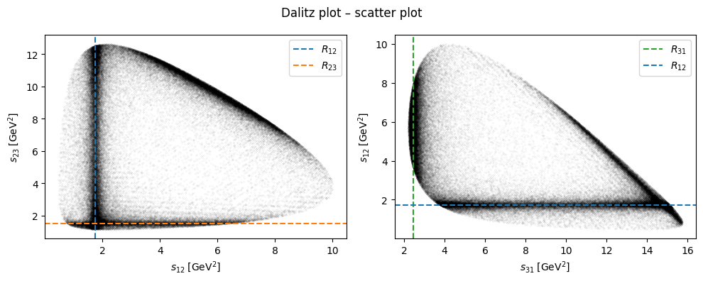
    url="https://indico.ific.uv.es/event/6803/contributions/21220/attachments/11209/15511/Three-particles-2.dat",
    path="data/Three-particles-2.dat",
    md5="831aee9fd925c43e8630edc6783ab28d",
    quiet=True,
    verify=False,
)
data2 = np.loadtxt(filename2)
pa, p1, p2, p3 = (data2[i::4].T for i in range(n_final_state + 1))

p0 = p1 + p2 + p3
m0 = mass(p0)
print(f"{m0.mean():.4g} +/- {m0.std():.4g}")

3.346 +/- 4.992e-07

Show code cell source

Hide code cell source

from IPython.display import Math

for i, p in enumerate([p0, p1, p2, p3]):
    display(Math(Rf"m_{i} = {mass(p).mean():.3g}\text{{ GeV}}"))

display(Math(Rf"m_{{a}} = {mass(pa).mean():.3g}\text{{ GeV}}"))

\[\displaystyle m_0 = 3.35\text{ GeV}\]

\[\displaystyle m_1 = 0.548\text{ GeV}\]

\[\displaystyle m_2 = 0.135\text{ GeV}\]

\[\displaystyle m_3 = 0.938\text{ GeV}\]

\[\displaystyle m_{a} = 0\text{ GeV}\]

Identify final state particles

Hide code cell source

from particle import Particle


def find_candidates(m: float, delta: float = 0.001) -> list[Particle]:
    return Particle.findall(lambda p: (m - delta) < 1e-3 * p.mass < (m + delta))


m1 = mass(p1).mean()
m2 = mass(p2).mean()
m3 = mass(p3).mean()
particles = tuple(find_candidates(m.mean())[0] for m in [m1, m2, m3])

src = R"\text{Final state: }" + ", ".join(f"{p.latex_name}" for p in particles)
Math(src)

\[\displaystyle \text{Final state: }\eta, \pi^{0}, p\]

This is again a photon \(\gamma\) hitting a target that produces a meson \(\eta\), pion \(\pi^0\), and proton \(p\).

s12 = mass_squared(p1 + p2)
s23 = mass_squared(p2 + p3)
s31 = mass_squared(p3 + p1)

m12 = mass(p1 + p2)
m23 = mass(p2 + p3)
m31 = mass(p3 + p1)

Show code cell source

Hide code cell source

import matplotlib.pyplot as plt

fig, ax = plt.subplots()
fig.suptitle("Dalitz plot – 2D histogram")
ax.hist2d(s12, s23, bins=100, cmin=1)
ax.set_xlabel(R"$s_{12}\;\left[\mathrm{GeV}^2\right]$")
ax.set_ylabel(R"$s_{23}\;\left[\mathrm{GeV}^2\right]$")
fig.tight_layout()
plt.show()

Show code cell source

Hide code cell source

fig, (ax1, ax2) = plt.subplots(figsize=(10, 4), ncols=2)
fig.suptitle("Dalitz plot – scatter plot")
ax1.scatter(s12, s23, c="black", s=1e-3)
ax1.set_xlabel(R"$s_{12}\;\left[\mathrm{GeV}^2\right]$")
ax1.set_ylabel(R"$s_{23}\;\left[\mathrm{GeV}^2\right]$")
ax1.axvline(R12, c="C0", ls="dashed", label="$R_{12}$")
ax1.axhline(R23, c="C1", ls="dashed", label="$R_{23}$")
ax1.legend()
ax2.scatter(s31, s12, c="black", s=1e-3)
ax2.set_xlabel(R"$s_{31}\;\left[\mathrm{GeV}^2\right]$")
ax2.set_ylabel(R"$s_{12}\;\left[\mathrm{GeV}^2\right]$")
ax2.axvline(R31, c="C2", ls="dashed", label="$R_{31}$")
ax2.axhline(R12, c="C0", ls="dashed", label="$R_{12}$")
ax2.legend()
fig.tight_layout()
plt.show()