Lecture 12 – Phase space simulation

How to perform a phase space simulation with Python?

Prepare the notebook by importing numpy, matplotlib.pyplot, and pylorentz and download the data file (CSV format) from Google Drive.

Import Python libraries

Hide code cell content

import matplotlib.pyplot as plt
import numpy as np
import phasespace
import tensorflow as tf
from pylorentz import Momentum4

WARNING: All log messages before absl::InitializeLog() is called are written to STDERR
I0000 00:00:1776092960.398773    3202 port.cc:153] oneDNN custom operations are on. You may see slightly different numerical results due to floating-point round-off errors from different computation orders. To turn them off, set the environment variable `TF_ENABLE_ONEDNN_OPTS=0`.
I0000 00:00:1776092960.399325    3202 cudart_stub.cc:31] Could not find cuda drivers on your machine, GPU will not be used.

WARNING: All log messages before absl::InitializeLog() is called are written to STDERR
I0000 00:00:1776092964.334628    3202 port.cc:153] oneDNN custom operations are on. You may see slightly different numerical results due to floating-point round-off errors from different computation orders. To turn them off, set the environment variable `TF_ENABLE_ONEDNN_OPTS=0`.
I0000 00:00:1776092964.334984    3202 cudart_stub.cc:31] Could not find cuda drivers on your machine, GPU will not be used.

Two-body decay

Let’s start with a simple two body decay at rest: \(B^0\rightarrow K^+\pi^-\).

B0_MASS = 5279.65
PION_MASS = 139.57018
KAON_MASS = 493.677
n_events = 100_000

decay = phasespace.nbody_decay(B0_MASS, [PION_MASS, KAON_MASS])
weights, four_momenta = decay.generate(n_events=n_events)

The simulation produces a dictionary (four_momenta) of tf.Tensor objects. Each object can be addressed with particles['p_i'], where i is the number of the \(i\)-th generated particle.

four_momenta

{'p_0': <tf.Tensor: shape=(100000, 4), dtype=float64, numpy=
 array([[-1986.4861371 , -1461.00868163,   869.97416587,  2618.58901417],
        [ -252.48780472,  -959.95868687, -2419.14402588,  2618.58901417],
        [ -762.0351893 , -1612.83248745,  1911.96295144,  2618.58901417],
        ...,
        [  190.79244115, -2282.20828645,  1262.00323758,  2618.58901417],
        [-2207.53128195,   113.58952403,  1396.93652298,  2618.58901417],
        [-2527.40828772,   155.65208927,  -652.31002157,  2618.58901417]],
       shape=(100000, 4))>,
 'p_1': <tf.Tensor: shape=(100000, 4), dtype=float64, numpy=
 array([[ 1986.4861371 ,  1461.00868163,  -869.97416587,  2661.06098583],
        [  252.48780472,   959.95868687,  2419.14402588,  2661.06098583],
        [  762.0351893 ,  1612.83248745, -1911.96295144,  2661.06098583],
        ...,
        [ -190.79244115,  2282.20828645, -1262.00323758,  2661.06098583],
        [ 2207.53128195,  -113.58952403, -1396.93652298,  2661.06098583],
        [ 2527.40828772,  -155.65208927,   652.31002157,  2661.06098583]],
       shape=(100000, 4))>}

Each tf.Tensor can be converted to a NumPy array, which can then be converted to a pylorentz.

def to_lorentz(p: tf.Tensor) -> Momentum4:
    p = p.numpy().T
    return Momentum4(p[3], *p[:3])

pion = to_lorentz(four_momenta["p_0"])
kaon = to_lorentz(four_momenta["p_1"])

These objects can be used to do kinematic computations. Let’s first verify that the invariant mass of the kaon+pion system corresponds to the mass of the mother \(B^0\):

B0 = pion + kaon
np.testing.assert_almost_equal(B0.m.mean(), B0_MASS)

Let’s also plot the momentum components of the two daugther particles.

Show code cell source

Hide code cell source

fig, ax = plt.subplots(1, 4, tight_layout=True, figsize=(11, 3.5))
ax[0].hist(B0.m, bins=100, color="CornFlowerBlue", range=(5279, 5280))
ax[0].set_xlabel(R"i.m.($\pi$K) [MeV/$c^2$]")
ax[0].set_title("(pion-kaon) i.m. \n")

ax[1].hist(kaon.p_x, bins=70, color="lightcoral", hatch="//")
ax[1].hist(
    pion.p_x,
    bins=70,
    color="springgreen",
    histtype="barstacked",
    hatch="\\",
    alpha=0.5,
)
ax[1].set_xlabel("$p_x$ [MeV/$c$]")
ax[1].set_title("x mom. component \n")

ax[2].hist(kaon.p_y, bins=70, color="lightcoral", hatch="//")
ax[2].hist(
    pion.p_y,
    bins=70,
    color="springgreen",
    histtype="barstacked",
    hatch="\\",
    alpha=0.5,
)
ax[2].set_xlabel("$p_y$ [MeV/$c$]")
ax[2].set_title("y mom. component \n")

ax[3].hist(kaon.p_z, bins=70, color="lightcoral", hatch="//")
ax[3].hist(
    pion.p_z,
    bins=70,
    color="springgreen",
    histtype="barstacked",
    hatch="\\",
    alpha=0.5,
)
ax[3].set_xlabel("$p_z$ [MeV/$c$]")
ax[3].set_title("z mom. component \n")
plt.show()

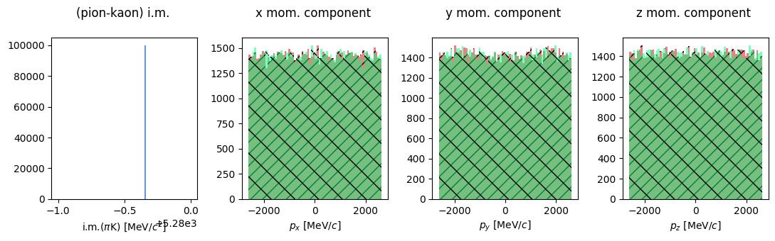
But it’s monochromatic!! of course it is… it’s a decay at rest. The momentum components are uniformly distributed in the available phase space.

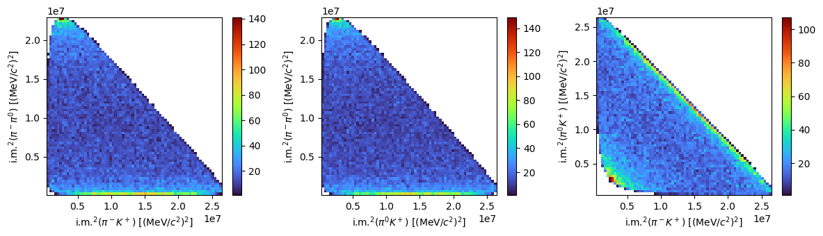
Three-body decay

Let’s consider now a three body decay like \(B^0\rightarrow K^+\pi^-\pi^0\) and repeat the plot of the relevant kinematic variables. We can also make Dalitz plots this time.

n_events = 50_000
PION0_MASS = 134.9766
decay = phasespace.nbody_decay(B0_MASS, [PION_MASS, PION0_MASS, KAON_MASS])
weights, four_momenta = decay.generate(n_events=n_events)

pim = to_lorentz(four_momenta["p_0"])
pi0 = to_lorentz(four_momenta["p_1"])
kaon = to_lorentz(four_momenta["p_2"])
s1 = (kaon + pim).m2
s2 = (kaon + pi0).m2
s3 = (pim + pi0).m2

Show code cell source

Hide code cell source

fig, ax = plt.subplots(1, 3, tight_layout=True, figsize=(12, 3.5))
f0 = ax[0].hist2d(s1, s3, bins=70, cmap="turbo", cmin=1)
fig.colorbar(f0[3], ax=ax[0])
ax[0].set_xlabel(R"i.m.$^2(\pi^-K^+)$ [(MeV/$c^2)^2]$")
ax[0].set_ylabel(R"i.m.$^2(\pi^-\pi^0)$ [(MeV/$c^2)^2]$")

f1 = ax[1].hist2d(s2, s3, bins=70, cmap="turbo", cmin=1)
fig.colorbar(f1[3], ax=ax[1])
ax[1].set_xlabel(R"i.m.$^2(\pi^0K^+)$ [(MeV/$c^2)^2]$")
ax[1].set_ylabel(R"i.m.$^2(\pi^-\pi^0)$ [(MeV/$c^2)^2]$")

f2 = ax[2].hist2d(s1, s2, bins=70, cmap="turbo", cmin=1)
fig.colorbar(f2[3], ax=ax[2])
ax[2].set_xlabel(R"i.m.$^2(\pi^-K^+)$ [(MeV/$c^2)^2]$")
ax[2].set_ylabel(R"i.m.$^2(\pi^0K^+)$ [(MeV/$c^2)^2]$")
plt.show()

Decay chain

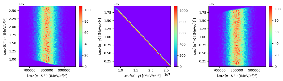
The phasespace package allows to treat also multiple decays. Let’s consider the \(B^0\rightarrow K^{\ast 0}\gamma\) decay, followed by \(K^{\ast 0}\rightarrow \pi^-K^+\). It can be simulated using the following procedure:

from phasespace import GenParticle

B0_MASS = 5279.65
K0STAR_MASS = 895.55
PION_MASS = 139.57018
KAON_MASS = 493.677
GAMMA_MASS = 0.0

Kp = GenParticle("K+", KAON_MASS)
pim = GenParticle("pi-", PION_MASS)
Kstar = GenParticle("KStar", K0STAR_MASS).set_children(Kp, pim)
gamma = GenParticle("gamma", GAMMA_MASS)
B0 = GenParticle("B0", B0_MASS).set_children(Kstar, gamma)

weights, four_momenta = B0.generate(n_events=100_000)

four_momenta

{'KStar': <tf.Tensor: shape=(100000, 4), dtype=float64, numpy=
 array([[ 1868.48465604, -1643.41544425,   617.56841329,  2715.77793272],
        [-1744.76874224, -1086.97452366,  1532.22335134,  2715.77793272],
        [  563.48050498,  2463.24534402,   433.99547584,  2715.77793272],
        ...,
        [ 2177.43070981,  -959.91894629,   954.35375929,  2715.77793272],
        [ 1362.27888445, -2098.49548894,   560.31500181,  2715.77793272],
        [  196.31784808, -1743.861922  ,  1869.18294366,  2715.77793272]],
       shape=(100000, 4))>,
 'gamma': <tf.Tensor: shape=(100000, 4), dtype=float64, numpy=
 array([[-1868.48465604,  1643.41544425,  -617.56841329,  2563.87206728],
        [ 1744.76874224,  1086.97452366, -1532.22335134,  2563.87206728],
        [ -563.48050498, -2463.24534402,  -433.99547584,  2563.87206728],
        ...,
        [-2177.43070981,   959.91894629,  -954.35375929,  2563.87206728],
        [-1362.27888445,  2098.49548894,  -560.31500181,  2563.87206728],
        [ -196.31784808,  1743.861922  , -1869.18294366,  2563.87206728]],
       shape=(100000, 4))>,
 'K+': <tf.Tensor: shape=(100000, 4), dtype=float64, numpy=
 array([[  997.10743658,  -710.85389953,   549.34661333,  1430.04726791],
        [-1649.86986991, -1094.05361059,  1268.0943014 ,  2402.24978469],
        [  507.8985522 ,  1102.09619517,   255.87178842,  1334.82744771],
        ...,
        [ 1341.67781   ,  -555.81366273,   278.26366015,  1558.90211958],
        [  727.18237936, -1546.94071181,   201.06391354,  1790.52044288],
        [  -75.33833887,  -720.1777328 ,   627.92111002,  1078.11582534]],
       shape=(100000, 4))>,
 'pi-': <tf.Tensor: shape=(100000, 4), dtype=float64, numpy=
 array([[  871.37721946,  -932.56154472,    68.22179995,  1285.73066481],
        [  -94.89887233,     7.07908693,   264.12904994,   313.52814803],
        [   55.58195279,  1361.14914885,   178.12368742,  1380.95048501],
        ...,
        [  835.75289981,  -404.10528356,   676.09009914,  1156.87581315],
        [  635.09650508,  -551.55477713,   359.25108827,   925.25748984],
        [  271.65618695, -1023.68418921,  1241.26183365,  1637.66210738]],
       shape=(100000, 4))>}

gamma = to_lorentz(four_momenta["gamma"])
pion = to_lorentz(four_momenta["pi-"])
kaon = to_lorentz(four_momenta["K+"])
Kstar = to_lorentz(four_momenta["KStar"])

Let’s build the Dalitz plots matching particle pairs. The particles measured in the final state are \(K^-,\; \pi^-\) and \(\gamma\).

s1 = (pion + kaon).m2
s2 = (gamma + kaon).m2
s3 = (gamma + pion).m2

Show code cell source

Hide code cell source

fig, ax = plt.subplots(1, 3, tight_layout=True, figsize=(12, 3.5))

f0 = ax[0].hist2d(s1, s2, bins=70, cmap="turbo")
fig.colorbar(f0[3], ax=ax[0])
ax[0].set_xlabel(R"i.m.$^2(\pi^-K^+)$ [(MeV/$c^2)^2]$")
ax[0].set_ylabel(R"i.m.$^2(K^+\gamma)$ [(MeV/$c^2)^2]$")

f1 = ax[1].hist2d(s2, s3, bins=70, cmap="turbo")
fig.colorbar(f1[3], ax=ax[1])
ax[1].set_xlabel(R"i.m.$^2(K^+\gamma)$ [(MeV/$c^2)^2]$")
ax[1].set_ylabel(R"i.m.$^2(\pi^-\gamma)$ [(MeV/$c^2)^2]$")

f2 = ax[2].hist2d(s1, s3, bins=70, cmap="turbo")
fig.colorbar(f2[3], ax=ax[2])
ax[2].set_xlabel(R"i.m.$^2(\pi^-K^+)$ [(MeV/$c^2)^2]$")
ax[2].set_ylabel(R"i.m.$^2(\pi^-\gamma)$ [(MeV/$c^2)^2]$")
plt.show()

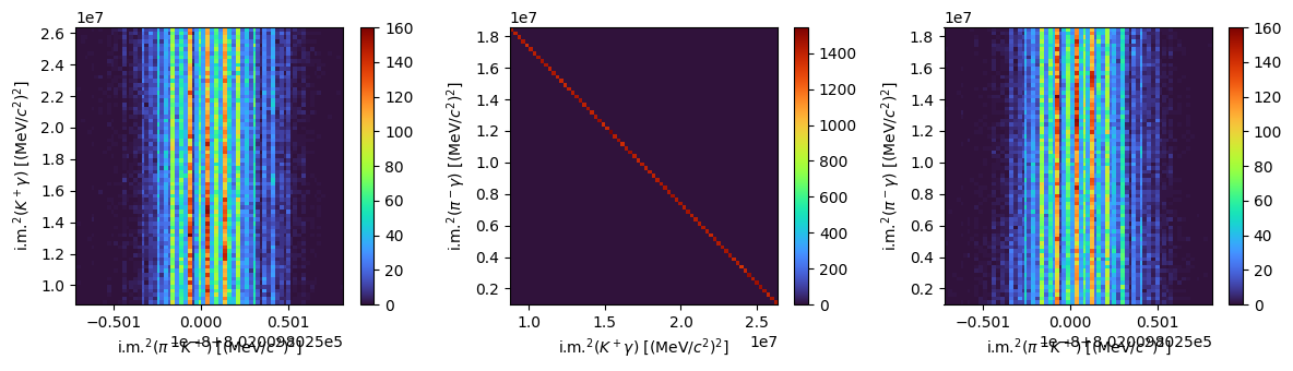
Width distribution

These distributions aren’t so interesting, because the masses of each particle are one fixed value. So let’s simulate a more realistic \(K^\ast\) particle; not monochromatic, but with a width of 47 MeV.[1] The mass is extracted from a Gaussian distribution centered at the B0_MASS value and with \(\sigma = 47/2.36 \sim 20\) MeV. See more info on how to do this with the phasespace package here.

import tensorflow as tf
import tensorflow_probability as tfp

K0STAR_WIDTH = 47 / 2.36


def kstar_mass(min_mass, max_mass, n_events):
    min_mass = tf.cast(min_mass, tf.float64)
    max_mass = tf.cast(max_mass, tf.float64)
    kstar_mass_cast = tf.cast(K0STAR_MASS, dtype=tf.float64)
    tf.cast(K0STAR_WIDTH, tf.float64)
    tf.broadcast_to(kstar_mass_cast, shape=(n_events,))
    return tfp.distributions.TruncatedNormal(
        loc=K0STAR_MASS,
        scale=K0STAR_WIDTH,
        low=min_mass,
        high=max_mass,
    ).sample()

K = GenParticle("K+", KAON_MASS)
pion = GenParticle("pi-", PION_MASS)
Kstar = GenParticle("KStar", kstar_mass).set_children(K, pion)
gamma = GenParticle("gamma", GAMMA_MASS)
B0 = GenParticle("B0", B0_MASS).set_children(Kstar, gamma)
weights, four_momenta = B0.generate(n_events=100_000)

gamma = to_lorentz(four_momenta["gamma"])
pion = to_lorentz(four_momenta["pi-"])
kaon = to_lorentz(four_momenta["K+"])
Kstar = to_lorentz(four_momenta["KStar"])

Now you have all the 4-vectors to plot the invariant mass distributions for the different steps of the decay chains.

s1 = (pion + kaon).m2
s2 = (gamma + kaon).m2
s3 = (gamma + pion).m2

Show code cell source

Hide code cell source

fig, ax = plt.subplots(1, 3, tight_layout=True, figsize=(12, 3.5))
f0 = ax[0].hist2d(s1, s2, bins=70, cmap="rainbow")
fig.colorbar(f0[3], ax=ax[0])
ax[0].set_xlabel(R"i.m.$^2(\pi^-K^+)$ [(MeV/$c^2)^2]$")
ax[0].set_ylabel(R"i.m.$^2(K^+\gamma)$ [(MeV/$c^2)^2]$")

f1 = ax[1].hist2d(s2, s3, bins=70, cmap="rainbow")
fig.colorbar(f1[3], ax=ax[1])
ax[1].set_xlabel(R"i.m.$^2(K^+\gamma)$ [(MeV/$c^2)^2]$")
ax[1].set_ylabel(R"i.m.$^2(\pi^-\gamma)$ [(MeV/$c^2)^2]$")

f2 = ax[2].hist2d(s1, s3, bins=70, cmap="rainbow")
fig.colorbar(f2[3], ax=ax[2])
ax[2].set_xlabel(R"i.m.$^2(\pi^-K^+)$ [(MeV/$c^2)^2]$")
ax[2].set_ylabel(R"i.m.$^2(\pi^-\gamma)$ [(MeV/$c^2)^2]$")
plt.show()

---

[1]

Do you remember the difference between a BW width and a Lorentzian FWHM? The widths you get out of the PDG booklet are FWHM’s.