Lecture 11 – Helicity formalism

Lecture 11 by Vincent Mathieu introduces spin into the Lorentz kinematics of Lecture 2 – Kinematics and treats it with the helicity formalism. The lecture comes with a data sample, Three-particles-3.dat, in which the spin of the resonances plays a role. In this notebook, we analyse this sample visually with a Dalitz plot and compare it with Three-particles-1.dat from Lecture 2 – Kinematics. We do not formulate an amplitude model for these data here.

Show code cell content

Hide code cell content

import warnings

import gdown
import matplotlib.pyplot as plt
import numpy as np
from IPython.display import Math
from particle import Particle

warnings.filterwarnings("ignore")

Reaction

As in Lecture 2 – Kinematics, each event in the data sample consists of the four-momenta \((E, p_x, p_y, p_z)\) of the beam particle \(a\) and the three final-state particles in the CoM frame. The four-momentum of the target \(b\) follows from four-momentum conservation.

def load_momenta(url: str, md5: str) -> tuple[np.ndarray, ...]:
    filename = gdown.cached_download(
        url=url,
        path=f"data/{url.rsplit('/', maxsplit=1)[-1]}",
        hash=f"md5:{md5}",
        quiet=True,
        verify=False,
    )
    data = np.loadtxt(filename)
    pa, p1, p2, p3 = (data[i::4].T for i in range(4))
    pb = p1 + p2 + p3 - pa
    return pa, pb, p1, p2, p3


pa, pb, p1, p2, p3 = load_momenta(
    url="https://indico.ific.uv.es/event/6803/contributions/21223/attachments/11221/15563/Three-particles-3.dat",
    md5="75fedf381f9b62d3210ff200fc63165f",
)
p0 = p1 + p2 + p3

The masses of the particles identify the reaction. Here, \(m_0\) is the invariant mass of the final state, that is, the CoM energy \(\sqrt{s}\).

def mass(p: np.ndarray) -> np.ndarray:
    return np.sqrt(mass_squared(p))


def mass_squared(p: np.ndarray) -> np.ndarray:
    return p[0] ** 2 - np.sum(p[1:] ** 2, axis=0)

Show code cell source

Hide code cell source

Math(Rf"""
\begin{{array}}{{rcl}}
  m_a &=& {mass(pa).mean():.3g} \text{{ GeV}} \\
  m_b &=& {mass(pb).mean():.3g} \text{{ GeV}} \\
  m_0 &=& {mass(p0).mean():.3g} \text{{ GeV}} \\
  m_1 &=& {mass(p1).mean():.3g} \text{{ GeV}} \\
  m_2 &=& {mass(p2).mean():.3g} \text{{ GeV}} \\
  m_3 &=& {mass(p3).mean():.3g} \text{{ GeV}}
\end{{array}}
""")

\[\begin{split}\displaystyle \begin{array}{rcl} m_a &=& 0 \text{ GeV} \\ m_b &=& 0.938 \text{ GeV} \\ m_0 &=& 4.1 \text{ GeV} \\ m_1 &=& 0.548 \text{ GeV} \\ m_2 &=& 0.135 \text{ GeV} \\ m_3 &=& 0.938 \text{ GeV} \end{array} \end{split}\]

We look up particles with these masses using the particle package. The gluon is excluded, because it is massless like the photon.

Show code cell source

Hide code cell source

def find_candidates(
    m_in_gev: float, delta_in_gev: float = 0.001, charge: float | None = None
) -> list[Particle]:
    def identify(p: Particle) -> bool:
        if p.pdgid == 21:
            return False
        if charge is not None and p.charge != charge:
            return False
        mass_in_gev = 1e-3 * p.mass
        return m_in_gev - delta_in_gev < mass_in_gev < m_in_gev + delta_in_gev

    return Particle.findall(identify)


initial_state = (
    find_candidates(mass(pa).mean(), delta_in_gev=1e-4)[0],
    find_candidates(mass(pb).mean())[0],
)
final_state = tuple(find_candidates(mass(p).mean())[0] for p in (p1, p2, p3))
Math(Rf"""
\begin{{array}}{{rl}}
  \text{{Incoming:}} & {", ".join(p.latex_name for p in initial_state)} \\
  \text{{Outgoing:}} & {", ".join(p.latex_name for p in final_state)}
\end{{array}}
""")

\[\begin{split}\displaystyle \begin{array}{rl} \text{Incoming:} & \gamma, p \\ \text{Outgoing:} & \eta, \pi^{0}, p \end{array} \end{split}\]

So this is the same reaction as in Three-particles-1.dat: a photon \(\gamma\) hitting a proton \(p\), producing an \(\eta\) meson, a pion \(\pi^0\), and a proton \(p\), at the same CoM energy of \(\sqrt{s} \approx 4.1\text{ GeV}\). The two samples can therefore be compared directly.

Dalitz plot

We plot two of the invariant masses squared \(s_{ij} = (p_i + p_j)^2\) against each other and estimate the positions \(R_{ij}\) of the resonance bands from the peaks in the distributions of \(s_{12}\), \(s_{23}\), and \(s_{31}\).

Show code cell source

Hide code cell source

COLORS = {"12": "C0", "23": "C1", "31": "C2"}


def find_peak(s: np.ndarray, bins: int = 200) -> float:
    counts, edges = np.histogram(s, bins=bins)
    i = counts.argmax()
    return (edges[i] + edges[i + 1]) / 2


def axis_label(ij: str) -> str:
    return Rf"$s_{{{ij}}}\;\left[\mathrm{{GeV}}^2\right]$"


def plot_dalitz(s: dict[str, np.ndarray], peaks: dict[str, float]) -> None:
    fig, (ax1, ax2, ax3) = plt.subplots(figsize=(12, 4), ncols=3)
    fig.suptitle("Dalitz plot")
    ax1.hist2d(s["12"], s["23"], bins=100, cmin=1)
    ax1.set_xlabel(axis_label("12"))
    ax1.set_ylabel(axis_label("23"))
    for ax, x, y in [(ax2, "12", "23"), (ax3, "31", "12")]:
        ax.scatter(s[x], s[y], c="black", s=1e-3, rasterized=True)
        ax.set_xlabel(axis_label(x))
        ax.set_ylabel(axis_label(y))
        ax.axvline(peaks[x], c=COLORS[x], ls="dashed", label=f"$R_{{{x}}}$")
        ax.axhline(peaks[y], c=COLORS[y], ls="dashed", label=f"$R_{{{y}}}$")
        ax.legend()
    fig.tight_layout()
    plt.show()


def plot_projections(s: dict[str, np.ndarray], peaks: dict[str, float]) -> None:
    fig, axes = plt.subplots(figsize=(12, 4), ncols=3)
    fig.suptitle("Distributions of $s_{12}$, $s_{23}$, and $s_{31}$")
    for ax, ij in zip(axes, s, strict=True):
        ax.hist(s[ij], bins=100, color="black", histtype="step")
        ax.set_xlabel(axis_label(ij))
        ax.set_ylabel("counts")
        ax.axvline(peaks[ij], c=COLORS[ij], ls="dashed", label=f"$R_{{{ij}}}$")
        ax.legend()
    fig.tight_layout()
    plt.show()

s = {
    "12": mass_squared(p1 + p2),
    "23": mass_squared(p2 + p3),
    "31": mass_squared(p3 + p1),
}
peaks = {ij: find_peak(s_ij) for ij, s_ij in s.items()}
{ij: round(float(np.sqrt(r)), 3) for ij, r in peaks.items()}

{'12': 1.317, '23': 1.237, '31': 1.564}

Show code cell source

Hide code cell source

plot_dalitz(s, peaks)

Show code cell source

Hide code cell source

plot_projections(s, peaks)

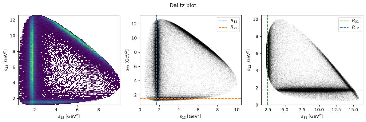
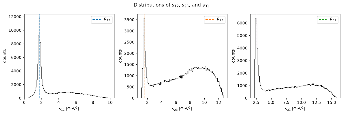
The candidates for the resonances \(R_{12} \to \eta\pi^0\), \(R_{23} \to \pi^0 p\), and \(R_{31} \to p\eta\) are:

find_candidates(np.sqrt(peaks["12"]), delta_in_gev=0.01, charge=0)

[<Particle: name="a(2)(1320)0", pdgid=115, mass=1318.2 ± 0.6 MeV>,
 <Particle: name="Xi0", pdgid=3322, mass=1314.86 ± 0.20 MeV>,
 <Particle: name="Xi~0", pdgid=-3322, mass=1314.86 ± 0.20 MeV>]

find_candidates(np.sqrt(peaks["23"]), delta_in_gev=0.01, charge=+1)

[<Particle: name="Delta(1232)~+", pdgid=-1114, mass=1232.0 ± 2.0 MeV>,
 <Particle: name="Delta(1232)+", pdgid=2214, mass=1232.0 ± 2.0 MeV>,
 <Particle: name="b(1)(1235)+", pdgid=10213, mass=1230 ± 3 MeV>,
 <Particle: name="a(1)(1260)+", pdgid=20213, mass=1230 ± 40 MeV>]

[
    p
    for p in find_candidates(np.sqrt(peaks["31"]), delta_in_gev=0.05, charge=+1)
    if p.pdgid > 0 and np.isclose(p.I, 1 / 2)
]

[<Particle: name="N(1520)+", pdgid=2124, mass=1515 ± 5 MeV>,
 <Particle: name="N(1535)+", pdgid=22212, mass=1530 ± 15 MeV>]

Following the same reasoning as in Lecture 2 – Kinematics, these are the same resonances as in Three-particles-1.dat: \(a_2(1320) \to \eta\pi^0\), \(\Delta(1232)^+ \to \pi^0 p\), and \(N(1535)^+ \to p\eta\). The bands in this Dalitz plot are more pronounced, however, and the events are distributed differently along them.

Spin effects

A resonance with nonzero spin generally produces an angular distribution of its decay products in its rest frame. Along a resonance band in the Dalitz plot, the other invariant masses are linear functions of the cosine of this decay angle, so an angular distribution shows up as a modulation of the event density along the band.

Three-particles-1.dat describes the same reaction at the same energy, but Lecture 2 – Kinematics shows that its event density along the bands is roughly flat. We therefore compare the normalised event density along each band in the two samples.

_, _, q1, q2, q3 = load_momenta(
    url="https://indico.ific.uv.es/event/6803/contributions/21220/attachments/11209/15504/Three-particles-1.dat",
    md5="a49ebfd97ae6a02023291df665ab924c",
)
s_ref = {
    "12": mass_squared(q1 + q2),
    "23": mass_squared(q2 + q3),
    "31": mass_squared(q3 + q1),
}

Show code cell source

Hide code cell source

def plot_band_comparison(
    s: dict[str, np.ndarray],
    s_ref: dict[str, np.ndarray],
    peaks: dict[str, float],
    width: float = 0.08,
) -> None:
    fig, axes = plt.subplots(figsize=(12, 4), ncols=3)
    fig.suptitle("Normalised event distributions along the resonance bands")
    for ax, (band, other) in zip(
        axes, [("12", "23"), ("23", "31"), ("31", "12")], strict=True
    ):
        for sample, label, color in [
            (s_ref, "Three-particles-1", "C7"),
            (s, "Three-particles-3", COLORS[band]),
        ]:
            selection = np.abs(sample[band] - peaks[band]) < width
            ax.hist(
                sample[other][selection],
                bins=60,
                color=color,
                density=True,
                histtype="step",
                label=label,
            )
        ax.set_title(Rf"$|s_{{{band}}} - R_{{{band}}}| < {width}\text{{ GeV}}^2$")
        ax.set_xlabel(axis_label(other))
        ax.set_yticks([])
        ax.legend(fontsize="small")
    fig.tight_layout()
    plt.show()


plot_band_comparison(s, s_ref, peaks)

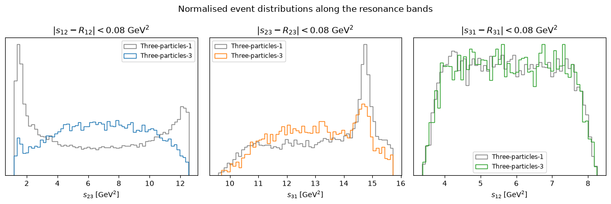
The difference is clearest along the \(a_2(1320)\) band. In Three-particles-1.dat, the event density is flat except at the ends of the band, where it crosses the \(\Delta(1232)\) and \(N(1535)\) bands. In Three-particles-3.dat, the density is largest in the middle of the band and drops towards its ends, which correspond to forward and backward decay angles. Such a modulation is what we expect from the decay of a resonance with nonzero spin, like the \(a_2(1320)\), which has \(J=2\). The \(\Delta(1232)\) band shows a weaker modulation of the same kind. The \(N(1535)\) band looks the same in both samples, which is consistent with its spin \(J=1/2\): the decay of an unpolarized spin-1/2 resonance into \(p\eta\) is isotropic.

To determine the spins and helicity couplings quantitatively, one would fit an amplitude model in the helicity formalism to these data.