Amplitude model with sympy#
This section is a follow-up of the previous chapter, Reaction and Models, to formulate the amplitude model for the \(\gamma p \to \eta\pi^0 p\) channel example symbolically. See TR‑033 for a purely numerical tutorial.
The model we want to implement is
\[\begin{split}
\begin{array}{rcl}
I &=& \left|A^{12} + A^{23} + A^{31}\right|^2 \\
A^{12} &=& \frac{\sum a_m Y_2^m (\Omega_1)}{s_{12}-m^2_{a_2}+im_{a_2} \Gamma_{a_2}} \\
A^{23} &=& \frac{\sum b_m Y_1^m (\Omega_2)}{s_{23}-m^2_{\Delta^+}+im_{\Delta^+} \Gamma_{\Delta^+}} \\
A^{31} &=& \frac{c_0}{s_{31}-m^2_{N^*}+im_{N^*} \Gamma_{N^*}} \,,
\end{array}
\end{split}\]
where \(1=\eta\), \(2=\pi^0\), and \(3=p\).
Model implementation#
l_max = 2
\(A^{12}\)#
s12, m_a2, gamma_a2, l12 = sp.symbols(r"s_{12} m_{a_2} \Gamma_{a_2} l_{12}")
theta1, phi1 = sp.symbols("theta_1 phi_1")
a = sp.IndexedBase("a")
m = sp.symbols("m", cls=sp.Idx)
A12 = sp.Sum(a[m] * sp.Ynm(l12, m, theta1, phi1), (m, -l12, l12)) / (
    s12 - m_a2**2 + sp.I * m_a2 * gamma_a2
)
A12
\[\displaystyle \frac{\sum_{m=- l_{12}}^{l_{12}} Y_{l_{12}}^{m}\left(\theta_{1},\phi_{1}\right) {a}_{m}}{i \Gamma_{a_2} m_{a_2} - m_{a_2}^{2} + s_{12}}\]
A12_funcs = [
    sp.lambdify(
        [s12, *(a[j] for j in range(-l_max, l_max + 1)), m_a2, gamma_a2, theta1, phi1],
        expr=A12.subs(l12, i).doit().expand(func=True),
    )
    for i in range(l_max + 1)
]
\(A^{23}\)#
s23, m_delta, gamma_delta, l23 = sp.symbols(
    r"s_{23} m_{\Delta^+} \Gamma_{\Delta^+} l_{23}"
)
b = sp.IndexedBase("b")
m = sp.symbols("m", cls=sp.Idx)
theta2, phi2 = sp.symbols("theta_2 phi_2")
A23 = sp.Sum(b[m] * sp.Ynm(l23, m, theta2, phi2), (m, -l23, l23)) / (
    s23 - m_delta**2 + sp.I * m_delta * gamma_delta
)
A23
\[\displaystyle \frac{\sum_{m=- l_{23}}^{l_{23}} Y_{l_{23}}^{m}\left(\theta_{2},\phi_{2}\right) {b}_{m}}{i \Gamma_{\Delta^+} m_{\Delta^+} - \left(m_{\Delta^+}\right)^{2} + s_{23}}\]
A23_funcs = [
    sp.lambdify(
        [
            s23,
            *(b[j] for j in range(-l_max, l_max + 1)),
            m_delta,
            gamma_delta,
            theta2,
            phi2,
        ],
        A23.subs(l23, i).doit().expand(func=True),
    )
    for i in range(l_max + 1)
]
\(A^{31}\)#
c = sp.IndexedBase("c")
s31, m_nstar, gamma_nstar = sp.symbols(r"s_{31} m_{N^*} \Gamma_{N^*}")
theta3, phi3, l31 = sp.symbols("theta_3 phi_3 l_{31}")
A31 = sp.Sum(c[m] * sp.Ynm(l31, m, theta3, phi3), (m, -l31, l31)) / (
    s31 - m_nstar**2 + sp.I * m_nstar * gamma_nstar
)
A31
\[\displaystyle \frac{\sum_{m=- l_{31}}^{l_{31}} Y_{l_{31}}^{m}\left(\theta_{3},\phi_{3}\right) {c}_{m}}{i \Gamma_{N^*} m_{N^*} - \left(m_{N^*}\right)^{2} + s_{31}}\]
A31_funcs = [
    sp.lambdify(
        [
            s31,
            *(c[j] for j in range(-l_max, l_max + 1)),
            m_nstar,
            gamma_nstar,
            theta3,
            phi3,
        ],
        A31.subs(l31, i).doit().expand(func=True),
    )
    for i in range(l_max + 1)
]
\(I = |A|^2 = |A^{12}+A^{23}+A^{31}|^2\)#
intensity_expr = sp.Abs(A12 + A23 + A31) ** 2
intensity_expr
\[\displaystyle \left|{\frac{\sum_{m=- l_{12}}^{l_{12}} Y_{l_{12}}^{m}\left(\theta_{1},\phi_{1}\right) {a}_{m}}{i \Gamma_{a_2} m_{a_2} - m_{a_2}^{2} + s_{12}} + \frac{\sum_{m=- l_{23}}^{l_{23}} Y_{l_{23}}^{m}\left(\theta_{2},\phi_{2}\right) {b}_{m}}{i \Gamma_{\Delta^+} m_{\Delta^+} - \left(m_{\Delta^+}\right)^{2} + s_{23}} + \frac{\sum_{m=- l_{31}}^{l_{31}} Y_{l_{31}}^{m}\left(\theta_{3},\phi_{3}\right) {c}_{m}}{i \Gamma_{N^*} m_{N^*} - \left(m_{N^*}\right)^{2} + s_{31}}}\right|^{2}\]
Phase Space Generation#
Mass for \(p\gamma\) system
E_lab_gamma = 8.5
m_proton = 0.938
m_0 = np.sqrt(2 * E_lab_gamma * m_proton + m_proton**2)
m_eta = 0.548
m_pi = 0.135
m_0
np.float64(4.101931740046389)
rng = TFUniformRealNumberGenerator(seed=0)
phsp_generator = TFPhaseSpaceGenerator(
    initial_state_mass=m_0,
    final_state_masses={1: m_eta, 2: m_pi, 3: m_proton},
)
phsp_momenta = phsp_generator.generate(500_000, rng)
Kinematic variables#
p1 = FourMomentumSymbol("p1", shape=[])
p2 = FourMomentumSymbol("p2", shape=[])
p3 = FourMomentumSymbol("p3", shape=[])
p12 = ArraySum(p1, p2)
p23 = ArraySum(p2, p3)
p31 = ArraySum(p3, p1)

theta1_expr, phi1_expr = formulate_helicity_angles(p1, p2)
theta2_expr, phi2_expr = formulate_helicity_angles(p2, p3)
theta3_expr, phi3_expr = formulate_helicity_angles(p3, p1)

s12_expr = SquaredInvariantMass(p12)
s23_expr = SquaredInvariantMass(p23)
s31_expr = SquaredInvariantMass(p31)
\[\begin{split}\begin{aligned}
\theta_{1} \;&=\; \theta\left(\boldsymbol{B_z}\left(\frac{\left|\vec{{p}_{12}}\right|}{E\left({p}_{12}\right)}\right) \boldsymbol{R_y}\left(- \theta\left({p}_{12}\right)\right) \boldsymbol{R_z}\left(- \phi\left({p}_{12}\right)\right) p_{1}\right) \\
\theta_{2} \;&=\; \theta\left(\boldsymbol{B_z}\left(\frac{\left|\vec{{p}_{23}}\right|}{E\left({p}_{23}\right)}\right) \boldsymbol{R_y}\left(- \theta\left({p}_{23}\right)\right) \boldsymbol{R_z}\left(- \phi\left({p}_{23}\right)\right) p_{2}\right) \\
\theta_{3} \;&=\; \theta\left(\boldsymbol{B_z}\left(\frac{\left|\vec{{p}_{31}}\right|}{E\left({p}_{31}\right)}\right) \boldsymbol{R_y}\left(- \theta\left({p}_{31}\right)\right) \boldsymbol{R_z}\left(- \phi\left({p}_{31}\right)\right) p_{3}\right) \\
\phi_{1} \;&=\; \phi\left(\boldsymbol{B_z}\left(\frac{\left|\vec{{p}_{12}}\right|}{E\left({p}_{12}\right)}\right) \boldsymbol{R_y}\left(- \theta\left({p}_{12}\right)\right) \boldsymbol{R_z}\left(- \phi\left({p}_{12}\right)\right) p_{1}\right) \\
\phi_{2} \;&=\; \phi\left(\boldsymbol{B_z}\left(\frac{\left|\vec{{p}_{23}}\right|}{E\left({p}_{23}\right)}\right) \boldsymbol{R_y}\left(- \theta\left({p}_{23}\right)\right) \boldsymbol{R_z}\left(- \phi\left({p}_{23}\right)\right) p_{2}\right) \\
\phi_{3} \;&=\; \phi\left(\boldsymbol{B_z}\left(\frac{\left|\vec{{p}_{31}}\right|}{E\left({p}_{31}\right)}\right) \boldsymbol{R_y}\left(- \theta\left({p}_{31}\right)\right) \boldsymbol{R_z}\left(- \phi\left({p}_{31}\right)\right) p_{3}\right) \\
s_{12} \;&=\; m_{{p}_{12}}^2 \\
s_{23} \;&=\; m_{{p}_{23}}^2 \\
s_{31} \;&=\; m_{{p}_{31}}^2 \\
\end{aligned}\end{split}\]
helicity_transformer = SympyDataTransformer.from_sympy(
    kinematic_variables, backend="jax"
)
phsp = helicity_transformer(phsp_momenta)
list(phsp)
['theta_1',
 'theta_2',
 'theta_3',
 'phi_1',
 'phi_2',
 'phi_3',
 's_{12}',
 's_{23}',
 's_{31}']
Parameters#
Note
The mass and width of each resonance is customized to make the resonance bands in the Dalitz plot more visible.
Visualization#
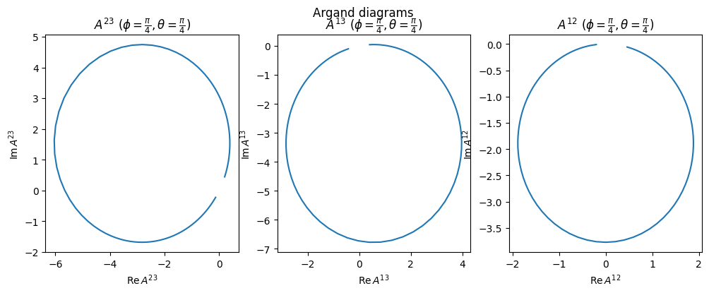
Model components#
phi = np.pi / 4
theta = np.pi / 4
s_values = np.linspace(0, 5, num=500)
A12_values = A12_funcs[2](s_values, *a_vals, m_a2_val, gamma_a2_val, theta, phi)
A23_values = A23_funcs[1](s_values, *b_vals, m_delta_val, gamma_delta_val, theta, phi)
A31_values = A31_funcs[0](s_values, *c_vals, m_nstar_val, gamma_nstar_val, theta, phi)
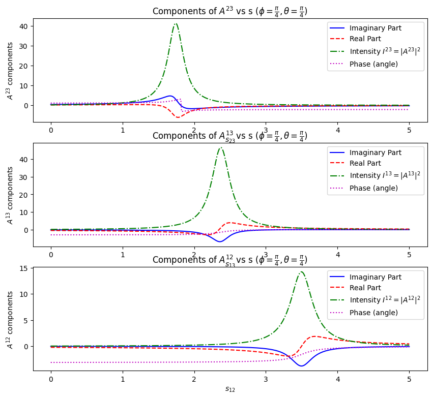
Unitarity is preserved in each of the subsystems (assuming fixed \(\phi,\theta\)), because we assume there is only one resonance in the subsystem.
Dalitz Plot#
intensity_funcs = np.array([
    [
        [
            create_parametrized_function(
                expression=intensity_expr
                .xreplace({l12: i, l23: j, l31: k})
                .doit()
                .expand(func=True),
                parameters=parameters_default,
                backend="jax",
            )
            for i in range(l_max + 1)
        ]
        for j in range(l_max + 1)
    ]
    for k in range(l_max + 1)
])
intensity_funcs.shape
(3, 3, 3)
%matplotlib widget
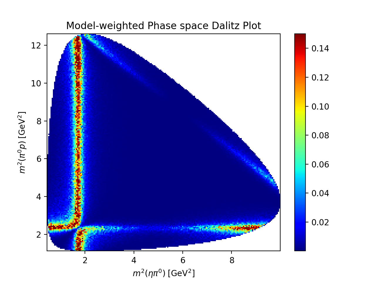
Projection#
