Lecture 6 – n̅ p

How to build and plot invariant masses of particle pairs and Dalitz plot for a reaction with three particles in the final state.

Prepare the notebook with the preambles for the inclusion of pandas, numpy and matplotlib.pyplot:

import matplotlib.pyplot as plt
import numpy as np
import pandas as pd

Download data Hide code cell source

import gdown

output_path = gdown.cached_download(
    url="https://drive.google.com/uc?id=17J4rrO-NHL8whkd7hjELhJbCoanoaqam",
    path="data/lecture6-nbarp-data.csv",
    md5="5ff45076c9d921aa0c9c803b8d2d8958",
    quiet=True,
)
data = pd.read_csv(output_path)

/opt/hostedtoolcache/Python/3.10.14/x64/lib/python3.10/site-packages/gdown/cached_download.py:102: FutureWarning: md5 is deprecated in favor of hash. Please use hash='md5:xxx...' instead.
  warnings.warn(

Inspect the data file and format. The file contains the 4-momenta of the particles of the reaction \(\bar n p \rightarrow \pi^+_1\pi^+_2\pi^-_3\), the last column corresponds to the 3rd component of the antineutron momentum (up to 300 MeV/c), which travels along the \(z\) axis

data.head()

	p1x	p1y	p1z	E1	p2x	p2y	p2z	E2	p3x	p3y	p3z	E3	pnbar
0	-0.649042	-0.462925	0.057760	0.811400	0.467449	-0.076535	0.248084	0.552622	0.184921	0.542265	0.101577	0.598368	0.407442
1	0.202017	-0.331041	-0.180710	0.450038	0.472889	0.469358	0.289029	0.739553	-0.684486	-0.139534	0.282087	0.766187	0.390522
2	0.131898	-0.111253	0.063348	0.230795	0.587119	0.420368	0.409048	0.841556	-0.715388	-0.309328	-0.252149	0.830976	0.220276
3	0.338881	-0.809633	0.106584	0.895090	0.088779	0.166919	0.040559	0.238469	-0.418469	0.641379	0.173450	0.797526	0.320725
4	-0.442309	0.269700	0.121178	0.550035	0.858318	-0.264391	0.039060	0.909735	-0.420124	-0.010746	0.112709	0.456948	0.273031

The columns headers present some trailing blanks, that must be dropped to be able to use correctly the DataFormat structure (if not, they deliver an error message). To do so, the str.strip() function must be used beforehand to reformat the column shape. In the following commands in the cell, columns are shown, overall with the data.columns command, and per single variable (like data.p2x). If the format is correct, no error should appear.

data.columns = data.columns.str.strip()
data.p2x

0        0.467449
1        0.472889
2        0.587119
3        0.088779
4        0.858318
           ...   
11892    0.462751
11893    0.431008
11894   -0.286882
11895   -0.166609
11896    0.327122
Name: p2x, Length: 11897, dtype: float64

Evaluate the invariant masses (squared and linear) for particle pairs. Every particle is defined by its four momentum \(\tilde p = (\vec p, E = \sqrt{p^2+m^2})\) with metric \((-, -, -, +)\). The invariant mass of a system of two particles \((a,b)\) is the module of the sum of their 4-momenta: \(i.m. = \sqrt{(\tilde{p_a}+\tilde{p_b})^2} = \sqrt{(E_a+E_b)^2 - |\vec{p_a}+\vec{p_b}|^2}\).

invariant_massSquared12 = (
    (data.E1 + data.E2) ** 2
    - (data.p1x + data.p2x) ** 2
    - (data.p1y + data.p2y) ** 2
    - (data.p1z + data.p2z) ** 2
)
invariant_mass12 = np.sqrt(invariant_massSquared12)
invariant_massSquared13 = (
    (data.E1 + data.E3) ** 2
    - (data.p1x + data.p3x) ** 2
    - (data.p1y + data.p3y) ** 2
    - (data.p1z + data.p3z) ** 2
)
invariant_mass13 = np.sqrt(invariant_massSquared13)
invariant_massSquared23 = (
    (data.E3 + data.E2) ** 2
    - (data.p3x + data.p2x) ** 2
    - (data.p3y + data.p2y) ** 2
    - (data.p3z + data.p2z) ** 2
)
invariant_mass23 = np.sqrt(invariant_massSquared23)

Look at the evaluated invariant masses to make sure they are different for different pion pairs

invariant_mass13

0        1.319225
1        1.007328
2        0.757867
3        1.658881
4        0.385310
           ...   
11892    1.212907
11893    0.805537
11894    1.541400
11895    1.248125
11896    1.319253
Length: 11897, dtype: float64

invariant_mass23

0        0.748348
1        1.336983
2        1.656491
3        0.515213
4        1.255816
           ...   
11892    1.459364
11893    0.837026
11894    0.711648
11895    1.119557
11896    0.975024
Length: 11897, dtype: float64

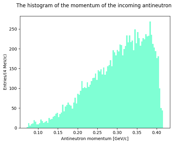
Let’s plot the evaluated invariant masses. First, though, let’s plot the antineutron momentum to see how the distribution looks like.

Show code cell source Hide code cell source

plt.hist(data.pnbar, bins=100, color="aquamarine")
plt.xlabel("Antineutron momentum [GeV/c]")
plt.ylabel("Entries/(4 MeV/c)")
plt.title("The histogram of the momentum of the incoming antineutron \n")
plt.show()

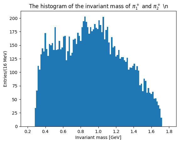
Let’s plot now the invariant masses distributions for the three pion pairs:

Show code cell source Hide code cell source

# plot the histogram pi1pi2 (both are pi+)
plt.hist(invariant_mass12, bins=100, range=(0.2, 1.8))
plt.xlabel("Invariant mass [GeV]")
plt.ylabel("Entries/(16 MeV)")
plt.title(R"The histogram of the invariant mass of $\pi_1^+$ and $\pi_2^+$ \n")
plt.show()

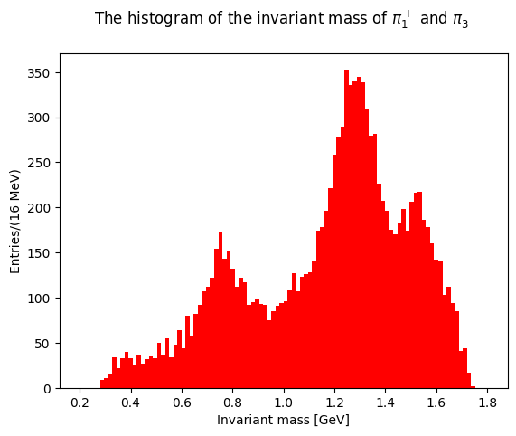
Show code cell source Hide code cell source

# plot the histogram pi1pi3 (both are pi+)
plt.hist(invariant_mass13, bins=100, color="red", range=(0.2, 1.8))
plt.xlabel("Invariant mass [GeV]")
plt.ylabel("Entries/(16 MeV)")
plt.title("The histogram of the invariant mass of $\\pi_1^+$ and $\\pi_3^-$\n")
plt.show()

Show code cell source Hide code cell source

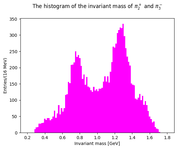
# plot the histogram pi2pi3 (both are pi+)
plt.hist(invariant_mass23, bins=100, color="magenta", range=(0.2, 1.8))
plt.xlabel("Invariant mass [GeV]")
plt.ylabel("Entries/(16 MeV)")
plt.title("The histogram of the invariant mass of $\\pi_2^+$ and $\\pi_3^-$\n")
plt.show()

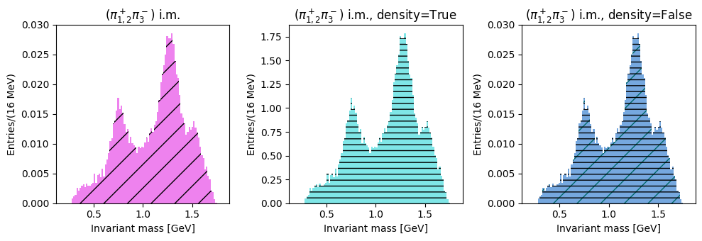
The last two plots can be cumulated in the same distribution, with two entries per event: this takes into account different combination of pions with opposite charges

Show code cell source Hide code cell source

im_merged = pd.concat([invariant_mass23, invariant_mass13])
# normalize to 1
merged_weights = np.ones_like(im_merged.values) / float(len(im_merged))
# two equivalent ways to plot the histograms with two entries per event normalized to 1
fig, ax = plt.subplots(1, 3, tight_layout=True, figsize=(10, 3.5))
ax[0].hist(
    im_merged,
    bins=100,
    weights=merged_weights,
    color="Violet",
    histtype="stepfilled",
    hatch="/",
    range=(0.2, 1.8),
)
ax[0].set_xlabel("Invariant mass [GeV]")
ax[0].set_ylabel("Entries/(16 MeV)")
ax[0].set_title(R"$(\pi_{1,2}^+\pi_3^-)$ i.m.")
ax[1].hist(
    im_merged,
    bins=100,
    weights=merged_weights,
    density=True,
    color="DarkTurquoise",
    histtype="stepfilled",
    alpha=0.5,
    stacked=True,
    hatch="--",
    range=(0.2, 1.8),
)
ax[1].set_xlabel("Invariant mass [GeV]")
ax[1].set_ylabel("Entries/(16 MeV)")
ax[1].set_title(R"$(\pi_{1,2}^+\pi_3^-)$ i.m., density=True")
ax[2].hist(
    im_merged,
    bins=100,
    weights=merged_weights,
    color="Violet",
    hatch="/",
    range=(0.2, 1.8),
)
ax[2].hist(
    im_merged,
    bins=100,
    weights=merged_weights,
    density=False,
    color="DarkTurquoise",
    alpha=0.5,
    stacked=True,
    hatch="--",
    range=(0.2, 1.8),
)
ax[2].set_xlabel("Invariant mass [GeV]")
ax[2].set_ylabel("Entries/(16 MeV)")
ax[2].set_title(R"$(\pi_{1,2}^+\pi_3^-)$ i.m., density=False")
plt.show()

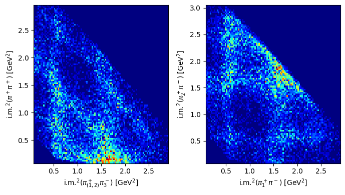
2D distributions: Dalitz plots

Show code cell source Hide code cell source

fig, ax = plt.subplots(1, 2, tight_layout=True, figsize=(7, 4))
ax[0].hist2d(invariant_massSquared13, invariant_massSquared12, bins=100, cmap="jet")
ax[0].hist2d(invariant_massSquared23, invariant_massSquared12, bins=100, cmap="jet")
# ax[0].colorbar()
ax[0].set_xlabel(R"i.m.$^2(\pi^+_{(1,2)}\pi^-_{3}$) [GeV$^2$]")
ax[0].set_ylabel(R"i.m.$^2(\pi^+\pi^+$) [GeV$^2$]")
ax[1].hist2d(invariant_massSquared13, invariant_massSquared23, bins=100, cmap="jet")
ax[1].hist2d(invariant_massSquared23, invariant_massSquared13, bins=100, cmap="jet")
ax[1].set_xlabel(R"i.m.$^2(\pi^+_1\pi^-$) [GeV$^2$]")
ax[1].set_ylabel(R"i.m.$^2(\pi^+_2\pi^-$) [GeV$^2$]")
plt.show()

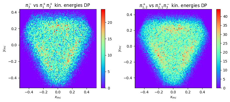
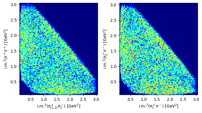
How do Dalitz plots look like with MonteCarlo generated data? Repeat the previous procedures with a new file, corresponding to generated data from the same reaction, and compare the shapes (statistics are different)

Download MC data Hide code cell source

path_mc = gdown.cached_download(
    url="https://drive.google.com/uc?id=1SarwF44sWSGbpn4PmBH3GLKIJJmN2lbS",
    path="data/lecture6-nbarp-mc.csv",
    md5="1221892fdcd056261ccb178748086679",
    quiet=True,
)
mc = pd.read_csv(path_mc)
mc.columns = mc.columns.str.strip()

/opt/hostedtoolcache/Python/3.10.14/x64/lib/python3.10/site-packages/gdown/cached_download.py:102: FutureWarning: md5 is deprecated in favor of hash. Please use hash='md5:xxx...' instead.
  warnings.warn(

invariant_massSquared12mc = (
    (mc.E1 + mc.E2) ** 2
    - (mc.p1x + mc.p2x) ** 2
    - (mc.p1y + mc.p2y) ** 2
    - (mc.p1z + mc.p2z) ** 2
)
invariant_massSquared13mc = (
    (mc.E1 + mc.E3) ** 2
    - (mc.p1x + mc.p3x) ** 2
    - (mc.p1y + mc.p3y) ** 2
    - (mc.p1z + mc.p3z) ** 2
)
invariant_massSquared23mc = (
    (mc.E3 + mc.E2) ** 2
    - (mc.p3x + mc.p2x) ** 2
    - (mc.p3y + mc.p2y) ** 2
    - (mc.p3z + mc.p2z) ** 2
)

Show code cell source Hide code cell source

fig, ax = plt.subplots(1, 2, tight_layout=True, figsize=(7, 4))
ax[0].hist2d(
    invariant_massSquared13mc, invariant_massSquared12mc, bins=100, cmap="jet"
)
ax[0].hist2d(
    invariant_massSquared23mc, invariant_massSquared12mc, bins=100, cmap="jet"
)
# ax[0].colorbar()
ax[0].set_xlabel(R"i.m.$^2(\pi^+_{(1,2)}\pi^-_{3}$) [GeV$^2$]")
ax[0].set_ylabel(R"i.m.$^2(\pi^+\pi^+$) [GeV$^2$]")
ax[1].hist2d(
    invariant_massSquared13mc, invariant_massSquared23mc, bins=100, cmap="jet"
)
ax[1].hist2d(
    invariant_massSquared23mc, invariant_massSquared13mc, bins=100, cmap="jet"
)
ax[1].set_xlabel(R"i.m.$^2(\pi^+_1\pi^-$) [GeV$^2$]")
ax[1].set_ylabel(R"i.m.$^2(\pi^+_2\pi^-$) [GeV$^2$]")
plt.show()

A Dalitz plot is defined as the phsyical region of the decay \(P\rightarrow a+b+c\) described by any variable linked to the total energies of two of the three particles \(a\) and \(b\) \(s_a=\sqrt{p^2_a+m^2_a}\) and \(s_b=\sqrt{p^2_b+m^2_b}\) by means of a linear transformation with constant Jacobian.

Therefore, other representations are possible. One is based on the particle kinetic energies, defined as follows: if \(T_a,\; T_b,\; T_c\) are the kinetic energies of the three particles and \(Q = T_a + T_b + T_c\) is their sum, one may use the two new coordinates \(x = (T_a - T_b)/\sqrt{3}\) and \(y = T_3 - Q/3\). Let’s try to make this plot with real and generated data.

# remember: all momenta are in GeV/c, so masses must be expressed in GeV/c^2
massChargedPion = 0.13957

T1 = np.sqrt(data.p1x**2 + data.p1y**2 + data.p1z**2) - massChargedPion
T2 = np.sqrt(data.p2x**2 + data.p2y**2 + data.p2z**2) - massChargedPion
T3 = np.sqrt(data.p3x**2 + data.p3y**2 + data.p3z**2) - massChargedPion
Q = T1 + T2 + T3
x = (T1 - T2) / np.sqrt(3)
y = T3 - Q / 3

Show code cell source Hide code cell source

plt.hist2d(x, y, bins=100, cmap="rainbow")
plt.colorbar()
plt.xlabel("x")
plt.ylabel("y")
plt.title(R"$\pi^-_{3}$ vs $\pi^+_{1}\pi^+_2$ kin. energies DP")
plt.show()

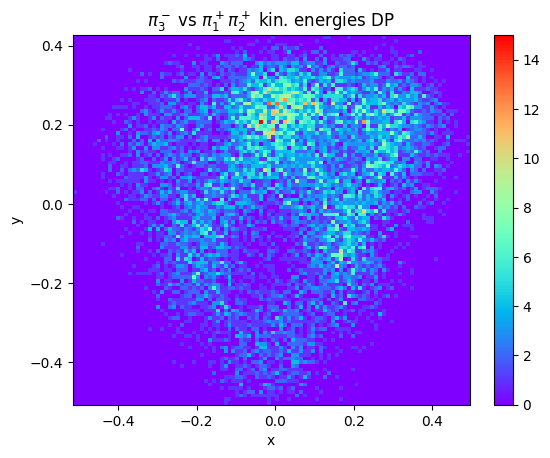
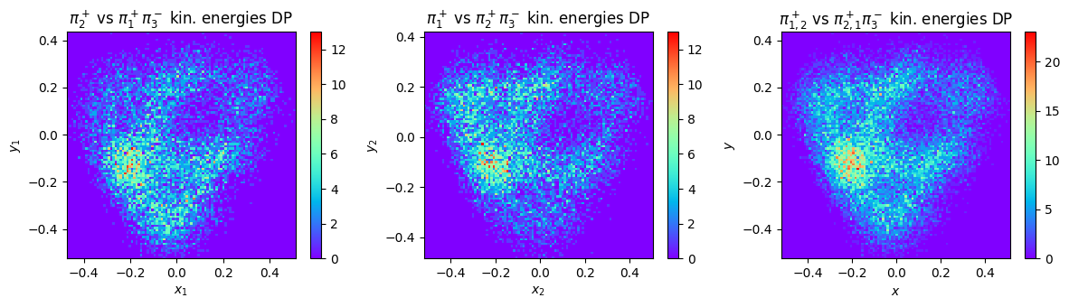
This plot of course requires a proper symmetrization over the charge combinations of the three pions.

Show code cell source Hide code cell source

# 1st combination (+-) vs (+)
x1 = (T1 - T3) / np.sqrt(3)
y1 = T2 - Q / 3
# 2nd combination (+-) vs (+)
x2 = (T2 - T3) / np.sqrt(3)
y2 = T1 - Q / 3

x2entries = pd.concat([x1, x2])
y2entries = pd.concat([y1, y2])

fig, ax = plt.subplots(1, 3, tight_layout=True, figsize=(12, 3.5))
h0 = ax[0].hist2d(x1, y1, bins=100, cmap="rainbow")
fig.colorbar(h0[3], ax=ax[0])
ax[0].set_xlabel("$x_1$")
ax[0].set_ylabel("$y_1$")
ax[0].set_title(R"$\pi^+_{2}$ vs $\pi^+_{1}\pi^-_3$ kin. energies DP")
h1 = ax[1].hist2d(x2, y2, bins=100, cmap="rainbow")
fig.colorbar(h1[3], ax=ax[1])
ax[1].set_xlabel("$x_2$")
ax[1].set_ylabel("$y_2$")
ax[1].set_title(R"$\pi^+_{1}$ vs $\pi^+_{2}\pi^-_3$ kin. energies DP")
# both combinations plotted on the same pad
h2 = ax[2].hist2d(x2entries, y2entries, bins=100, cmap="rainbow")
fig.colorbar(h2[3], ax=ax[2])
ax[2].set_xlabel("$x$")
ax[2].set_ylabel("$y$")
ax[2].set_title(R"$\pi^+_{1,2}$ vs $\pi^+_{2,1}\pi^-_3$ kin. energies DP")
plt.show()

Let’s repeat the calculations and produced for mc phase space events

Show code cell source Hide code cell source

T1mc = np.sqrt(mc.p1x**2 + mc.p1y**2 + mc.p1z**2) - massChargedPion
T2mc = np.sqrt(mc.p2x**2 + mc.p2y**2 + mc.p2z**2) - massChargedPion
T3mc = np.sqrt(mc.p3x**2 + mc.p3y**2 + mc.p3z**2) - massChargedPion
Qmc = T1mc + T2mc + T3mc
xmc = (T1mc - T2mc) / np.sqrt(3)
ymc = T3mc - Qmc / 3

# 1st combination (+-) vs (+)
x1mc = (T1mc - T3mc) / np.sqrt(3)
y1mc = T2mc - Qmc / 3
# 2nd combination (+-) vs (+)
x2mc = (T2mc - T3mc) / np.sqrt(3)
y2mc = T1mc - Qmc / 3
x2entriesmc = pd.concat([x1mc, x2mc])
y2entriesmc = pd.concat([y1mc, y2mc])

fig, ax = plt.subplots(1, 2, tight_layout=True, figsize=(9, 4))
h0 = ax[0].hist2d(xmc, ymc, bins=100, cmap="rainbow")
fig.colorbar(h0[3], ax=ax[0])
ax[0].set_xlabel("$x_{mc}$")
ax[0].set_ylabel("$y_{mc}$")
ax[0].set_title(R"$\pi^-_3$ vs $\pi^+_1\pi^+_2$ kin. energies DP")
h1 = ax[1].hist2d(x2entriesmc, y2entriesmc, bins=100, cmap="rainbow")
fig.colorbar(h1[3], ax=ax[1])
ax[1].set_xlabel("$x_{mc}$")
ax[1].set_ylabel("$y_{mc}$")
ax[1].set_title(R"$\pi^+_{1,2}$ vs $\pi^+_{2,1}\pi^-_3$ kin. energies DP")
plt.show()