Lecture 12 – γ p [solution]#
Invariant masses of particle pairs and Dalitz plots for another reaction with three particles in the final state \(\gamma p\rightarrow \pi^+\pi^-p\).
Prepare the notebook with the preambles for the inclusion of pandas, numpy and matplotlib.pyplot:
Import Python libraries
import gdown
import matplotlib.pyplot as plt
import numpy as np
import pandas as pd
from pylorentz import Momentum4
Download data
output_path = gdown.cached_download(
    url="https://drive.google.com/uc?id=1qiYjPbR5nx3_Sw7MXuUKhNAUpkXPoxYh",
    path="data/lecture6-gammap-data.csv",
    md5="38cf5bf915318df756a21a82ad9e4afa",
    quiet=True,
)
data = pd.read_csv(output_path)
data.columns = data.columns.str.strip()
data
/opt/hostedtoolcache/Python/3.10.14/x64/lib/python3.10/site-packages/gdown/cached_download.py:102: FutureWarning: md5 is deprecated in favor of hash. Please use hash='md5:xxx...' instead.
  warnings.warn(
| p1x | p1y | p1z | E1 | p2x | p2y | p2z | E2 | p3x | p3y | p3z | E3 | pgamma | helGamma | ||
|---|---|---|---|---|---|---|---|---|---|---|---|---|---|---|---|
| 0 | 0.517085 | 0.161989 | 0.731173 | 0.920732 | -0.254367 | 0.082889 | 0.495509 | 0.580189 | -0.259266 | -0.265152 | 0.445175 | 1.10275 | 1.657800 | -1 | |
| 1 | -0.216852 | -0.245333 | 0.107538 | 0.371878 | -0.183380 | 0.191897 | 0.145128 | 0.333213 | 0.389750 | 0.112110 | 0.790133 | 1.29195 | 1.044790 | -1 | |
| 2 | 0.197931 | 0.071432 | -0.010077 | 0.252778 | -0.111780 | -0.360482 | 0.367842 | 0.545221 | -0.090228 | 0.302313 | 0.724911 | 1.22694 | 1.095470 | -1 | |
| 3 | -0.505371 | -0.163949 | 0.450407 | 0.710395 | -0.141057 | 0.282404 | 1.186530 | 1.235730 | 0.679497 | -0.112014 | 0.729706 | 1.37371 | 2.388690 | -1 | |
| 4 | 0.260706 | -0.330303 | 0.385968 | 0.587839 | 0.163863 | 0.354007 | 0.286983 | 0.504031 | -0.490385 | -0.019313 | 0.879568 | 1.37653 | 1.454880 | 1 | |
| ... | ... | ... | ... | ... | ... | ... | ... | ... | ... | ... | ... | ... | ... | ... | ... |
| 701969 | 0.128575 | -0.018500 | 0.143663 | 0.238807 | 0.378718 | -0.051974 | 0.461311 | 0.615185 | -0.497148 | 0.087386 | 0.483961 | 1.17020 | 1.083930 | -1 | |
| 701970 | -0.262395 | -0.235015 | 0.024120 | 0.379712 | 0.330904 | -0.040001 | 0.751630 | 0.834003 | -0.095422 | 0.256882 | 0.695036 | 1.19938 | 1.492470 | 1 | |
| 701971 | -0.068621 | 0.111528 | -0.032843 | 0.194273 | -0.274412 | -0.101159 | 0.115541 | 0.344094 | 0.325894 | -0.006340 | 0.781223 | 1.26369 | 0.862625 | -1 | |
| 701972 | 0.297759 | -0.100136 | 0.766630 | 0.840194 | 0.034110 | 0.110721 | 0.409582 | 0.447991 | -0.472764 | -0.012095 | 0.440591 | 1.13935 | 2.200460 | -1 | |
| 701973 | 0.169067 | 0.426984 | 0.254915 | 0.543504 | -0.122702 | 0.017682 | -0.012514 | 0.187193 | -0.074462 | -0.430331 | 0.953283 | 1.40707 | 1.587060 | -1 |
701974 rows × 15 columns
The columns headers present some trailing blanks, that must be dropped to be able to use correctly the DataFormat structure (if not, they deliver an error message). To do so, the
str.strip()function must be used beforehand to reformat the column shape.
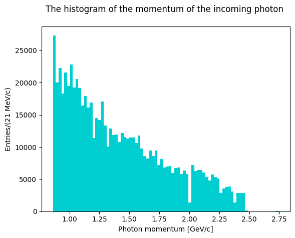
Inspect the data file and format. The file contains the 4-momenta of the particles of the reaction \(\gamma p \rightarrow \pi^+\pi^- p\), the last column corresponds to the 3rd component of the photon momentum (up to 2.5 GeV/c), which travels along the \(z\) axis. Since the target was made of HD, to select the data interacting on protons only a cut on the missing momentum of the reaction was made.
Invariant mass distributions#
Measured data#
Exercise 9
Evaluate the invariant masses (squared and linear) for particle pairs, in a similar way as done in the first example.
Solution to Exercise 9
# @title Solution
inv_mass_squared_12 = (
    (data.E1 + data.E2) ** 2
    - (data.p1x + data.p2x) ** 2
    - (data.p1y + data.p2y) ** 2
    - (data.p1z + data.p2z) ** 2
)
inv_mass_squared_13 = (
    (data.E1 + data.E3) ** 2
    - (data.p1x + data.p3x) ** 2
    - (data.p1y + data.p3y) ** 2
    - (data.p1z + data.p3z) ** 2
)
inv_mass_squared_23 = (
    (data.E3 + data.E2) ** 2
    - (data.p3x + data.p2x) ** 2
    - (data.p3y + data.p2y) ** 2
    - (data.p3z + data.p2z) ** 2
)
invariant_mass_12 = np.sqrt(inv_mass_squared_12)
invariant_mass_13 = np.sqrt(inv_mass_squared_13)
invariant_mass_23 = np.sqrt(inv_mass_squared_23)
Exercise 10
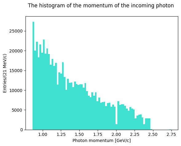
Plot the evaluated invariant masses. First, though, let’s plot the antineutron momentum to see how the distribution looks like.
Solution to Exercise 10
Show code cell source
# @title Solution
plt.hist(data.pgamma, bins=80, color="turquoise")
plt.xlabel("Photon momentum [GeV/c]")
plt.ylabel("Entries/(21 MeV/c)")
plt.title("The histogram of the momentum of the incoming photon \n")
plt.show()
Exercise 11
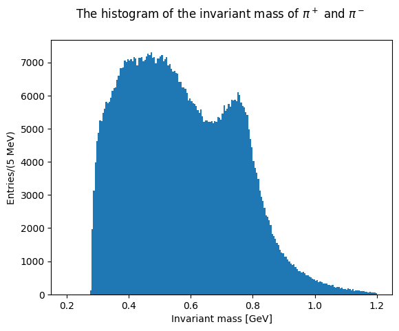
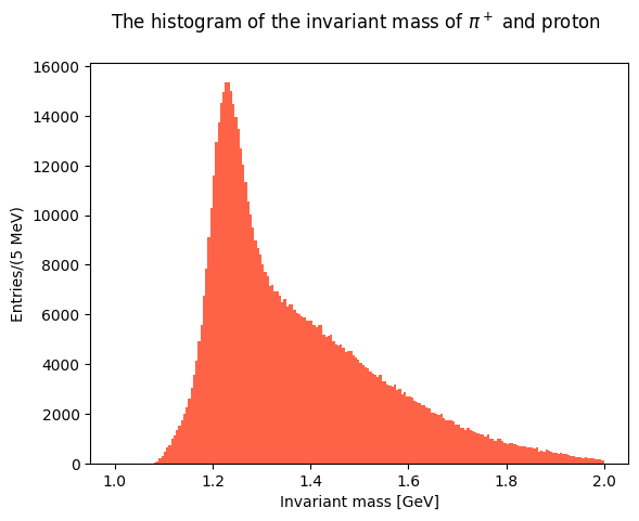
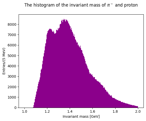
Now plot the invariant masses distributions for the three pion pairs.
Solution to Exercise 11
Show code cell source
# @title Solution
# plot the histogram pi+pi-
plt.hist(invariant_mass_12, bins=200, range=(0.2, 1.2))
plt.xlabel("Invariant mass [GeV]")
plt.ylabel("Entries/(5 MeV)")
plt.title("The histogram of the invariant mass of $\\pi^+$ and $\\pi^-$ \n")
plt.show()
Show code cell source
# @title Solution
# plot the histogram pi+proton
plt.hist(invariant_mass_13, bins=200, color="tomato", range=(1.0, 2.0))
plt.xlabel("Invariant mass [GeV]")
plt.ylabel("Entries/(5 MeV)")
plt.title("The histogram of the invariant mass of $\\pi^+$ and proton  \n")
plt.show()
Show code cell source
# @title Solution
# plot the histogram pi-proton
plt.hist(invariant_mass_23, bins=200, color="darkmagenta", range=(1.0, 2.0))
plt.xlabel("Invariant mass [GeV]")
plt.ylabel("Entries/(5 MeV)")
plt.title("The histogram of the invariant mass of $\\pi^-$ and proton \n")
plt.show()
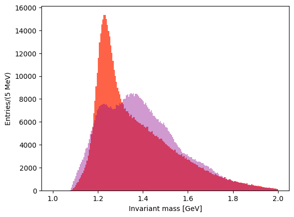
You can superimpose the two last plots to check the differences in the lineshapes of the two distributions.
Show code cell source
# @title Solution
plt.hist(invariant_mass_13, bins=200, color="tomato", range=(1.0, 2.0))
plt.hist(
    invariant_mass_23, bins=200, color="darkmagenta", alpha=0.4, range=(1.0, 2.0)
)
plt.xlabel("Invariant mass [GeV]")
plt.ylabel("Entries/(5 MeV)")
plt.show()
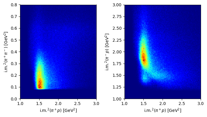
Exercise 12
Plot the distributions over the Dalitz plane.
Solution to Exercise 12
Show code cell source
# @title Solution
fig, ax = plt.subplots(1, 2, tight_layout=True, figsize=(7, 4))
ax[0].hist2d(
    inv_mass_squared_13,
    inv_mass_squared_12,
    bins=200,
    range=[[1.0, 3], [0.0, 0.8]],
    cmap="jet",
)
ax[0].set_xlabel(R"i.m.$^2(\pi^+p$) [GeV$^2$]")
ax[0].set_ylabel(R"i.m.$^2(\pi^+\pi^-$) [GeV$^2$]")
ax[1].hist2d(
    inv_mass_squared_13,
    inv_mass_squared_23,
    bins=200,
    range=[[1.0, 3], [1.0, 3.0]],
    cmap="jet",
)
ax[1].set_xlabel(R"i.m.$^2(\pi^+p$) [GeV$^2$]")
ax[1].set_ylabel(R"i.m.$^2(\pi^-p$) [GeV$^2$]")
plt.show()
Monte Carlo data#
How do Dalitz plots look like with MonteCarlo generated data? Repeat the previous procedures with a new file, corresponding to generated data from the same reaction, and compare the shapes (statistics are different)
Download MC data
path_mc = gdown.cached_download(
    url="https://drive.google.com/uc?id=11J0xaQLRMxzgQLXEhXZb_u4mnxp8RVPO",
    path="data/lecture6-gammap-mc.csv",
    md5="04152c69c802b13a55a3ffb3d07012d1",
    quiet=True,
)
mc = pd.read_csv(path_mc)
mc.columns = mc.columns.str.strip()
/opt/hostedtoolcache/Python/3.10.14/x64/lib/python3.10/site-packages/gdown/cached_download.py:102: FutureWarning: md5 is deprecated in favor of hash. Please use hash='md5:xxx...' instead.
  warnings.warn(
# @title Solution
inv_mass_squared_12_mc = (
    (mc.E1 + mc.E2) ** 2
    - (mc.p1x + mc.p2x) ** 2
    - (mc.p1y + mc.p2y) ** 2
    - (mc.p1z + mc.p2z) ** 2
)
inv_mass_squared_13_mc = (
    (mc.E1 + mc.E3) ** 2
    - (mc.p1x + mc.p3x) ** 2
    - (mc.p1y + mc.p3y) ** 2
    - (mc.p1z + mc.p3z) ** 2
)
inv_mass_squared_23_mc = (
    (mc.E3 + mc.E2) ** 2
    - (mc.p3x + mc.p2x) ** 2
    - (mc.p3y + mc.p2y) ** 2
    - (mc.p3z + mc.p2z) ** 2
)
The phase space simulation was done extracting the photon momentum from the real data distribution.
Show code cell source
# @title Solution
plt.hist(data.pgamma, bins=80, color="darkturquoise")
plt.xlabel("Photon momentum [GeV/c]")
plt.ylabel("Entries/(21 MeV/c)")
plt.title("The histogram of the momentum of the incoming photon \n")
plt.show()
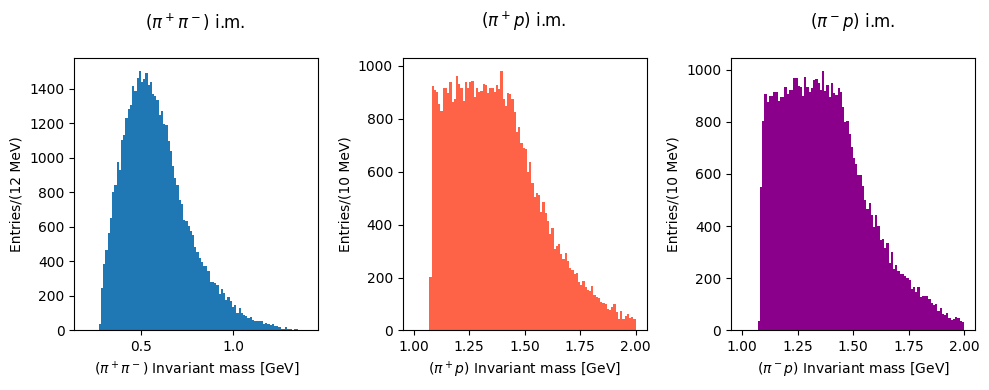
Let’s see the invariant masses histogram shapes using phase space Monte Carlo events.
Show code cell source
# @title Solution
fig, ax = plt.subplots(1, 3, tight_layout=True, figsize=(10, 4))

# plot the histogram pi+pi-
ax[0].hist(np.sqrt(inv_mass_squared_12_mc), bins=100, range=(0.2, 1.4))
ax[0].set_xlabel(R"($\pi^+\pi^-$) Invariant mass [GeV]")
ax[0].set_ylabel("Entries/(12 MeV)")
ax[0].set_title("($\\pi^+\\pi^-$) i.m. \n")
# plot the histogram pi+p
ax[1].hist(
    np.sqrt(inv_mass_squared_13_mc), color="tomato", bins=100, range=(1.0, 2.0)
)
ax[1].set_xlabel(R"($\pi^+p$) Invariant mass [GeV]")
ax[1].set_ylabel("Entries/(10 MeV)")
ax[1].set_title("($\\pi^+p$) i.m. \n")
# plot the histogram pi-pi-
ax[2].hist(
    np.sqrt(inv_mass_squared_23_mc), bins=100, color="darkmagenta", range=(1.0, 2.0)
)
ax[2].set_xlabel(R"($\pi^-p$) Invariant mass [GeV]")
ax[2].set_ylabel("Entries/(10 MeV)")
ax[2].set_title("($\\pi^-p$) i.m. \n")
plt.show()
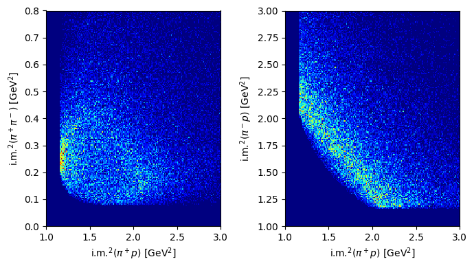
And now the Dalitz plots:
Show code cell source
# @title Solution
fig, ax = plt.subplots(1, 2, tight_layout=True, figsize=(7, 4))
ax[0].hist2d(
    inv_mass_squared_13_mc,
    inv_mass_squared_12_mc,
    bins=200,
    range=[[1.0, 3], [0.0, 0.8]],
    cmap="jet",
)
ax[0].set_xlabel(R"i.m.$^2(\pi^+p$) [GeV$^2$]")
ax[0].set_ylabel(R"i.m.$^2(\pi^+\pi^-$) [GeV$^2$]")
ax[1].hist2d(
    inv_mass_squared_13_mc,
    inv_mass_squared_23_mc,
    bins=200,
    range=[[1.0, 3], [1.0, 3.0]],
    cmap="jet",
)
ax[1].set_xlabel(R"i.m.$^2(\pi^+p$) [GeV$^2$]")
ax[1].set_ylabel(R"i.m.$^2(\pi^-p$) [GeV$^2$]")
plt.show()
Missing mass distributions#
Now, let’s take a look to the missing mass distribution (final - initial
state). Let’s start from the real data using the pylorentz package to build 4-vectors (first, work out the lecture12b-kinematics.ipynb notebook).
# final state
pip = Momentum4(data.E1, data.p1x, data.p1y, data.p1z)
pim = Momentum4(data.E2, data.p2x, data.p2y, data.p2z)
proton = Momentum4(data.E3, data.p3x, data.p3y, data.p3z)

# initial state
m_proton = 0.93827
n_events = len(data)
zeros = np.zeros(n_events)
ones = np.ones(n_events)
gamma = Momentum4(data.pgamma, zeros, zeros, data.pgamma)
target = Momentum4(m_proton * ones, zeros, zeros, zeros)
Show code cell source
init = gamma + target
final = pip + pim + proton
missingMomentum = final - init

plt.hist(missingMomentum.m2, bins=200, color="palegreen", range=(-0.02, 0.01))
plt.xlabel(R"Missing mass squared [$(\mathrm{GeV}/c^2)^2$]")
plt.ylabel(R"Entries/($5x10^{-5}\;(\mathrm{GeV}/c^2)^2$)")
plt.title("Missing momentum \n")
plt.show()
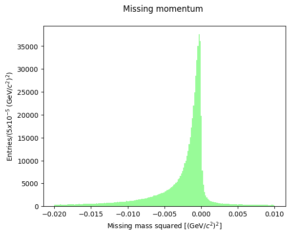
The missing mass square is always negative: this means that the total energy of the initial state exceeds the measured energy of the final state, so there is (likely) a missing particle which carries away some energy. We know that the reaction occurred on a HD molecule as a target: this means that a recoiling neutron is present in all cases when the reaction occurred on a deuteron nucleus: \(\gamma p(n)\rightarrow \pi^+\pi^- p (n)\). In this case, moreover, the hit proton is not at rest but it may have a momentum (called Fermi momentum) which, in the deuteron center-of-mass, is roughly distributed as a gaussian 50 MeV/c wide, with maximum at abouth 270 MeV/c. The missing mass momentum distribution shows the effect of the presence of a non-null Fermi momentum, and the possible contribution to the reaction kinematics of the spectator neutron.
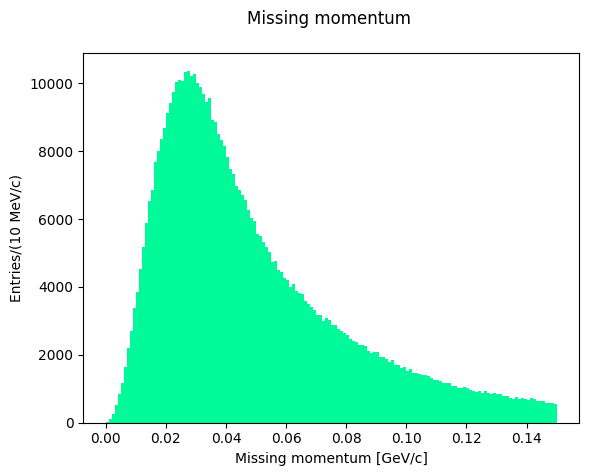
In the data selection procedure, the Fermi momentum was required not to exceed 100 MeV/c to preserve the condition that the neutron is a spectator in the reaction occurring on deuteron. Let’s see the shape of the missing momentum distribution:
Show code cell source
plt.hist(missingMomentum.p, bins=150, color="mediumspringgreen", range=(0.0, 0.150))
plt.xlabel("Missing momentum [GeV/c]")
plt.ylabel("Entries/(10 MeV/c)")
plt.title("Missing momentum \n")
plt.show()
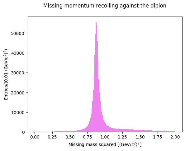
Let’s now consider the missing mass recoiling against the neutral dipion: in an exclusive reaction we expect it to peak at the proton mass. Is the PID selection of our sample acceptable?
Show code cell source
dipion = pip + pim
missingMomentumDipion = init - dipion

plt.hist(missingMomentumDipion.m2, bins=200, color="violet", range=(0.0, 2))
plt.xlabel(R"Missing mass squared [$(\mathrm{GeV}/c^2)^2$]")
plt.ylabel(R"Entries/($0.01\;(\mathrm{GeV}/c^2)^2$)")
plt.title("Missing momentum recoiling against the dipion\n")
plt.show()
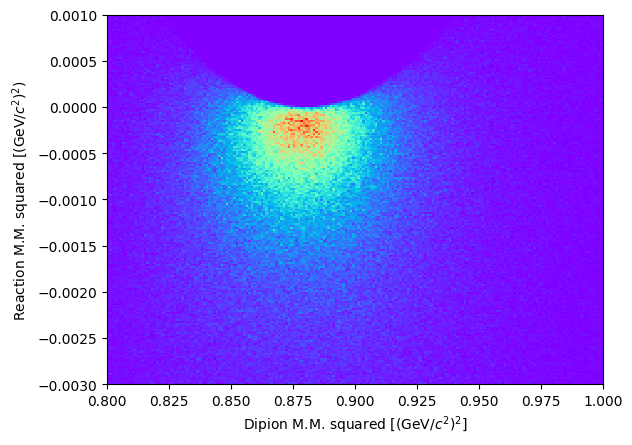
Let’s visualize the scatter plot of the two missing masses squared:
Show code cell source
fig = plt.figure()
plt.hist2d(
    missingMomentumDipion.m2,
    missingMomentum.m2,
    bins=200,
    range=[[0.80, 1.0], [-0.003, 0.001]],
    cmap="rainbow",
)
plt.xlabel(R"Dipion M.M. squared [$(\mathrm{GeV}/c^2)^2$]")
plt.ylabel(R"Reaction M.M. squared [$(\mathrm{GeV}/c^2)^2$)")
plt.show()
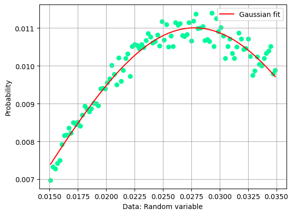
Let’s do some fits#
Which is the maximum of the missing momentum, and where is the peak of the missing mass distribution? Let’s attempt two fits with a single gaussian function.
Show code cell source
from scipy.optimize import curve_fit

# normalize the histogram to 1
low_edge = 0.015
up_edge = 0.035
hist, bin_edges = np.histogram(missingMomentum.p, 100, range=(low_edge, up_edge))
integral_hist = sum(hist)
hist = hist / integral_hist

n = hist.size
x_hist = np.zeros((n), dtype=float)
for ii in range(n):
    x_hist[ii] = (bin_edges[ii + 1] + bin_edges[ii]) / 2

y_hist = hist

# Calculating the Gaussian PDF values given Gaussian parameters and random variable X


def gaus(X, C, X_mean, sigma):
    return C * np.exp(-((X - X_mean) ** 2) / (2 * sigma**2))


mean = sum(x_hist * y_hist) / sum(y_hist)
sigma = sum(y_hist * (x_hist - mean) ** 2) / sum(y_hist)

# Gaussian least-square fitting process
param_optimised, param_covariance_matrix = curve_fit(
    gaus, x_hist, y_hist, p0=[max(y_hist), mean, sigma], maxfev=5000
)

# print fit Gaussian parameters
print("Fit parameters: ")
print("=====================================================")
print("C = ", param_optimised[0], "+-", np.sqrt(param_covariance_matrix[0, 0]))
print("X_mean =", param_optimised[1], "+-", np.sqrt(param_covariance_matrix[1, 1]))
print("sigma = ", param_optimised[2], "+-", np.sqrt(param_covariance_matrix[2, 2]))
print("\n")


# STEP 4: PLOTTING THE GAUSSIAN CURVE -----------------------------------------
fig = plt.figure()
x_hist_2 = np.linspace(np.min(x_hist), np.max(x_hist), 100)
# this plots the curve only
plt.plot(
    x_hist_2, gaus(x_hist_2, *param_optimised), color="red", label="Gaussian fit"
)
plt.legend()

# plot the experimental point of the portion of spectrum to be fitted
plt.scatter(x_hist, y_hist, color="mediumspringgreen")

# Normalise the histogram values
weights = np.ones_like(y_hist) / y_hist.size
# plt.hist(x_hist, weights=weights)
# plt.hist(x_hist)
# plt.hist(hist)


# setting the label,title and grid of the plot
plt.xlabel("Data: Random variable")
plt.ylabel("Probability")
plt.grid("on")
plt.show()
Fit parameters:
=====================================================
C =  0.011005709743577008 +- 3.732733551478205e-05
X_mean = 0.027786976736489354 +- 0.00012906543968641603
sigma =  0.014235101514555967 +- 0.0002582282909194536
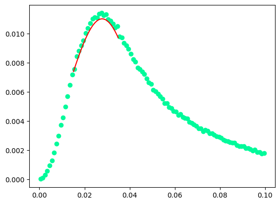
Show code cell source
# normalize the histogram to 1 and then to ratio of the maximum values
histfull, bin_edgesf = np.histogram(missingMomentum.p, 100, range=(0.0, 0.10))
n = histfull.size
xf_hist = np.zeros((n), dtype=float)
ilow = 0
iup = 0
# find the bin numbers corresponding to fitted histrogram edges
for ii in range(n):
    xf_hist[ii] = (bin_edgesf[ii + 1] + bin_edgesf[ii]) / 2
    # find the closest bin to edges
    if bin_edgesf[ii + 1] <= low_edge:
        ilow = ii
    if bin_edgesf[ii + 1] <= up_edge:
        iup = ii


integralFull = sum(histfull)
histfull = histfull / integralFull
yf_hist = histfull
histfull = histfull * np.max(y_hist) / np.max(yf_hist)
yf_hist = histfull

plt.scatter(xf_hist, yf_hist, color="mediumspringgreen")

x_hist_3 = np.linspace(np.min(x_hist), np.max(x_hist), 100)
plt.plot(x_hist_3, gaus(x_hist_3, *param_optimised), color="red")  # was 'r.:'
plt.show()
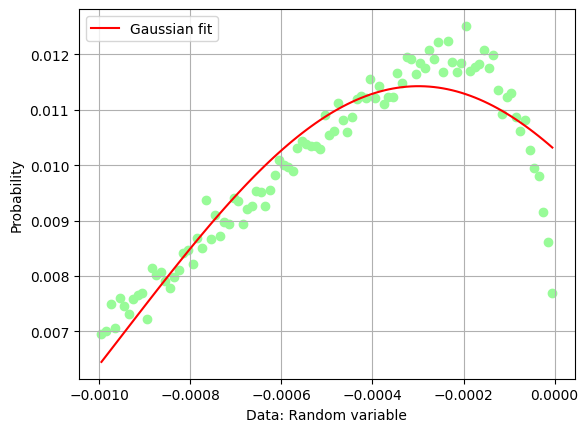
Show code cell source
# normalize the histogram to 1
low_edge = -0.001
up_edge = 0.0
hist, bin_edges = np.histogram(missingMomentum.m2, 100, range=(low_edge, up_edge))
integral_hist = sum(hist)
hist = hist / integral_hist

n = hist.size
x_hist = np.zeros((n), dtype=float)
for ii in range(n):
    x_hist[ii] = (bin_edges[ii + 1] + bin_edges[ii]) / 2

y_hist = hist
mean = sum(x_hist * y_hist) / sum(y_hist)
sigma = sum(y_hist * (x_hist - mean) ** 2) / sum(y_hist)
# Gaussian least-square fitting process
param_optimised, param_covariance_matrix = curve_fit(
    gaus, x_hist, y_hist, p0=[max(y_hist), mean, sigma], maxfev=5000
)

# print fit Gaussian parameters
print("Fit parameters: ")
print("=====================================================")
print("C = ", param_optimised[0], "+-", np.sqrt(param_covariance_matrix[0, 0]))
print("X_mean =", param_optimised[1], "+-", np.sqrt(param_covariance_matrix[1, 1]))
print("sigma = ", param_optimised[2], "+-", np.sqrt(param_covariance_matrix[2, 2]))
print("\n")

# save the values for later
mean1Fit = param_optimised[1]
sigma1Fit = param_optimised[2]

# STEP 4: PLOTTING THE GAUSSIAN CURVE -----------------------------------------
fig = plt.figure()
x_hist_2 = np.linspace(np.min(x_hist), np.max(x_hist), 100)
# this plots the curve only
plt.plot(
    x_hist_2, gaus(x_hist_2, *param_optimised), color="red", label="Gaussian fit"
)
plt.legend()

# plot the experimental point of the portion of spectrum to be fitted
plt.scatter(x_hist, y_hist, color="palegreen")

# setting the label,title and grid of the plot
plt.xlabel("Data: Random variable")
plt.ylabel("Probability")
plt.grid("on")
plt.show()
Fit parameters:
=====================================================
C =  0.011425786457275298 +- 7.980412291207278e-05
X_mean = -0.00029890467303904025 +- 1.4417745309981776e-05
sigma =  0.0006508651338504216 +- 2.1985899655909954e-05
Show code cell source
# normalize the histogram to 1 and then to ratio of the maximum values
histfull, bin_edgesf = np.histogram(missingMomentum.m2, 100, range=(-0.005, 0.005))
n = histfull.size
xf_hist = np.zeros((n), dtype=float)

# find the bin numbers
for ii in range(n):
    xf_hist[ii] = (bin_edgesf[ii + 1] + bin_edgesf[ii]) / 2

integralFull = sum(histfull)
histfull = histfull / integralFull
yf_hist = histfull
histfull = histfull * np.max(y_hist) / np.max(yf_hist)
yf_hist = histfull

plt.scatter(xf_hist, yf_hist, color="palegreen")
x_hist_3 = np.linspace(np.min(x_hist), np.max(x_hist), 100)
plt.plot(x_hist_3, gaus(x_hist_3, *param_optimised), color="red")
plt.show()
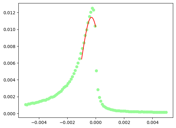
The fit of the missing mass peak is not really very good, one should add some sort of background on the left hand side of the peak, say a 3rd degree polynomial
Show code cell source
# normalize the histogram to 1
low_edge = -0.0007
up_edge = 0.0001
hist, bin_edges = np.histogram(missingMomentum.m2, 100, range=(low_edge, up_edge))
integral_hist = sum(hist)
hist = hist / integral_hist

n = hist.size
x_hist = np.zeros((n), dtype=float)
for ii in range(n):
    x_hist[ii] = (bin_edges[ii + 1] + bin_edges[ii]) / 2

y_hist = hist
mean = sum(x_hist * y_hist) / sum(y_hist)
sigma = sum(y_hist * (x_hist - mean) ** 2) / sum(y_hist)
# mean = mean1Fit
# sigma = sigma1Fit
P1 = 0.0
P2 = 0.0
P3 = 0.0
P4 = 0.0

# Calculating the Gaussian PDF values given Gaussian parameters and random variable X


def gausAndBCK(X, C, X_mean, sigma, P1, P2, P3, P4):
    return C * np.exp(-((X - X_mean) ** 2) / (2 * sigma**2)) + (
        P1 + P2 * X + P3 * X * X + P4 * X * X * X
    )


def BCK(X, P1, P2, P3, P4):
    return P1 + P2 * X + P3 * X * X + P4 * X * X * X


# Gaussian+BCK least-square fitting process
param_optimised, param_covariance_matrix = curve_fit(
    gausAndBCK,
    x_hist,
    y_hist,
    p0=[max(y_hist), mean, sigma, P1, P2, P3, P4],
    maxfev=10000,
)

# print fit Gaussian parameters
print("Fit parameters: ")
print("=====================================================")
print("C = ", param_optimised[0], "+-", np.sqrt(param_covariance_matrix[0, 0]))
print("X_mean =", param_optimised[1], "+-", np.sqrt(param_covariance_matrix[1, 1]))
print("sigma = ", param_optimised[2], "+-", np.sqrt(param_covariance_matrix[2, 2]))
print("\n")
print("missing mass at the peak ", np.sqrt(abs(param_optimised[1])), " GeV/c2 \n")

param_optimised_gauss = []
param_optimised_bck = []
param_optimised_gauss.append(param_optimised[0])
param_optimised_gauss.append(param_optimised[1])
param_optimised_gauss.append(param_optimised[2])
param_optimised_bck.append(param_optimised[3])
param_optimised_bck.append(param_optimised[4])
param_optimised_bck.append(param_optimised[5])
param_optimised_bck.append(param_optimised[6])

fig, ax = plt.subplots(1, 2, tight_layout=True, figsize=(7, 4))
x_hist_2 = np.linspace(np.min(x_hist), np.max(x_hist), 100)
# this plots the curve only
ax[0].plot(
    x_hist_2,
    gausAndBCK(x_hist_2, *param_optimised),
    color="red",
    label="Gaussian fit",
)
ax[0].plot(x_hist_2, gaus(x_hist_2, *param_optimised_gauss), color="cyan")
ax[0].plot(x_hist_2, BCK(x_hist_2, *param_optimised_bck), color="magenta")

# plot the experimental point of the portion of spectrum to be fitted
ax[0].scatter(x_hist, y_hist, color="palegreen")

# setting the label,title and grid of the plot

ax[0].set_xlabel("Data: Random variable")
ax[0].set_ylabel("Probability")

# full plot
histfull, bin_edgesf = np.histogram(missingMomentum.m2, 100, range=(-0.005, 0.005))
n = histfull.size
xf_hist = np.zeros((n), dtype=float)

# find the bin numbers
for ii in range(n):
    xf_hist[ii] = (bin_edgesf[ii + 1] + bin_edgesf[ii]) / 2

integralFull = sum(histfull)
histfull = histfull / integralFull
yf_hist = histfull
histfull = histfull * np.max(y_hist) / np.max(yf_hist)
yf_hist = histfull

plt.scatter(xf_hist, yf_hist, color="palegreen")
x_hist_3 = np.linspace(np.min(x_hist), np.max(x_hist), 100)
plt.plot(x_hist_3, gausAndBCK(x_hist_3, *param_optimised), color="red")
plt.show()
/tmp/ipykernel_2164/2314849554.py:37: OptimizeWarning: Covariance of the parameters could not be estimated
  param_optimised, param_covariance_matrix = curve_fit(
Fit parameters:
=====================================================
C =  0.012374654548228295 +- inf
X_mean = -0.0003200492404461684 +- inf
sigma =  5.5094292099376265e-09 +- inf


missing mass at the peak  0.017889920079367832  GeV/c2
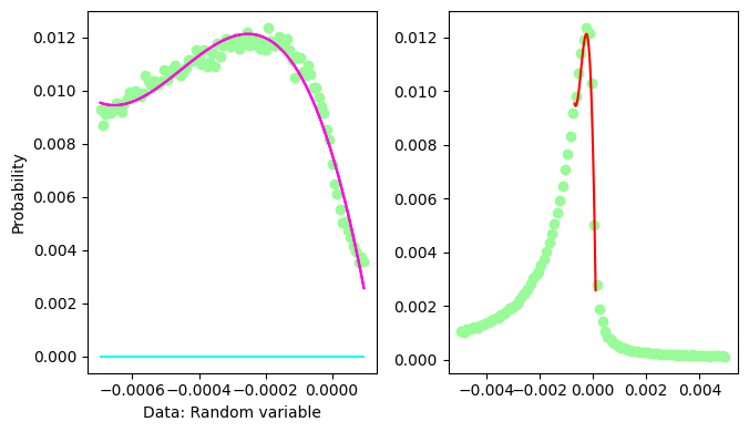
It looks like the Gaussian contribution is refused by the fit.
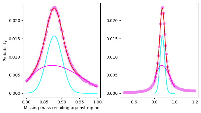
Let’s make a similar fit for the missing mass recoiling against the dipion:
Show code cell source
# normalize the histogram to 1
low_edge = 0.8
up_edge = 1.0
hist, bin_edges = np.histogram(
    missingMomentumDipion.m2, 100, range=(low_edge, up_edge)
)
integral_hist = np.sum(hist)
hist = hist / integral_hist

n = hist.size
x_hist = np.zeros((n), dtype=float)
for ii in range(n):
    x_hist[ii] = (bin_edges[ii + 1] + bin_edges[ii]) / 2

y_hist = hist
mean = sum(x_hist * y_hist) / sum(y_hist)
sigma = sum(y_hist * (x_hist - mean) ** 2) / sum(y_hist)
# mean = mean1Fit
# sigma = sigma1Fit
P1 = 0.0
P2 = 0.0
P3 = 0.0
P4 = 0.0

# Calculating the Gaussian PDF values given Gaussian parameters and random variable X


def gausAndBCK(X, C, X_mean, sigma, P1, P2, P3, P4):
    return C * np.exp(-((X - X_mean) ** 2) / (2 * sigma**2)) + (
        P1 + P2 * X + P3 * X * X + P4 * X * X * X
    )


def BCK(X, P1, P2, P3, P4):
    return P1 + P2 * X + P3 * X * X + P4 * X * X * X


# Gaussian+BCK least-square fitting process
param_optimised, param_covariance_matrix = curve_fit(
    gausAndBCK,
    x_hist,
    y_hist,
    p0=[max(y_hist), mean, sigma, P1, P2, P3, P4],
    maxfev=10000,
)

# print fit Gaussian parameters
print("Fit parameters: ")
print("=====================================================")
print("C = ", param_optimised[0], "+-", np.sqrt(param_covariance_matrix[0, 0]))
print("X_mean =", param_optimised[1], "+-", np.sqrt(param_covariance_matrix[1, 1]))
print("sigma = ", param_optimised[2], "+-", np.sqrt(param_covariance_matrix[2, 2]))
print("\n")
print("missing mass at the peak ", np.sqrt(abs(param_optimised[1])), " GeV/c2 \n")

param_optimised_gauss = []
param_optimised_bck = []
param_optimised_gauss.append(param_optimised[0])
param_optimised_gauss.append(param_optimised[1])
param_optimised_gauss.append(param_optimised[2])
param_optimised_bck.append(param_optimised[3])
param_optimised_bck.append(param_optimised[4])
param_optimised_bck.append(param_optimised[5])
param_optimised_bck.append(param_optimised[6])

fig, ax = plt.subplots(1, 2, tight_layout=True, figsize=(7, 4))
x_hist_2 = np.linspace(np.min(x_hist), np.max(x_hist), 100)
# this plots the curve only
ax[0].plot(
    x_hist_2,
    gausAndBCK(x_hist_2, *param_optimised),
    color="red",
    label="Gaussian fit",
)
ax[0].plot(x_hist_2, gaus(x_hist_2, *param_optimised_gauss), color="cyan")
ax[0].plot(x_hist_2, BCK(x_hist_2, *param_optimised_bck), color="magenta")

# plot the experimental point of the portion of spectrum to be fitted
ax[0].scatter(x_hist, y_hist, color="violet")

# setting the label,title and grid of the plot

ax[0].set_xlabel("Missing mass recoiling against dipion")
ax[0].set_ylabel("Probability")

# full plot
histfull, bin_edgesf = np.histogram(missingMomentumDipion.m2, 100, range=(0.5, 1.2))
n = histfull.size
xf_hist = np.zeros((n), dtype=float)

# find the bin numbers
for ii in range(n):
    xf_hist[ii] = (bin_edgesf[ii + 1] + bin_edgesf[ii]) / 2

integralFull = sum(histfull)
histfull = histfull / integralFull
yf_hist = histfull
histfull = histfull * np.max(y_hist) / np.max(yf_hist)
yf_hist = histfull

plt.scatter(xf_hist, yf_hist, color="violet")
x_hist_3 = np.linspace(np.min(x_hist), np.max(x_hist), 100)
plt.plot(x_hist_3, gausAndBCK(x_hist_3, *param_optimised), color="red")
plt.plot(x_hist_3, gaus(x_hist_3, *param_optimised_gauss), color="cyan")
plt.plot(x_hist_3, BCK(x_hist_3, *param_optimised_bck), color="magenta")
plt.show()
Fit parameters:
=====================================================
C =  0.01575028042415391 +- 0.00020064999359329676
X_mean = 0.8788503281352017 +- 0.0001461108225442943
sigma =  0.02245277193520005 +- 0.0002493807482134945


missing mass at the peak  0.9374701745310097  GeV/c2