Lecture 9 – Estimators#
Import Python libraries
import gdown
import matplotlib.pyplot as plt
import numpy as np
import scipy.optimize as opt
import scipy.stats as stats
from lmfit import Model
from lmfit.models import ExpressionModel
from matplotlib.colors import BoundaryNorm
from matplotlib.ticker import MaxNLocator
from scipy.stats import chi2, norm
Estimator Definition#
An estimator is a procedure applied to the data sample which gives a numerical value for a property of the parent population or a property/parameter of the parent distribution. Suppose that the quantity we want to measure is called \(a\). \(\hat{a}\) is an estimator.
Let’s consider an estimator \(\hat{a}\) to find the average height \(a\) of all students of the University on the basis of a sample N. Let’s consider the different estimators:
Add up all the heigths and divide by N
Add up the first 10 heights and divide by 10. Ignore the rest
Add up all the heigths and divide by N-1
Trow away the data and give 1.8 as answer
Add up the second, fourth, sixth,… heights and divide by N/2 for N even and (N-1)/2 for N odd
Consistent#
Consistent: \(\lim_{N\to\infty} \hat{a} = a\), that is you can get as close to the true value as you want, as long as you have a large enough data set. In the previous example 1 is consistent:
for \(N\) going to infinity \(\bar{x}\rightarrow\mu\): law of big numbers. 3 and 5 are also consistent since N-1 or N/2 make little difference when \(N\rightarrow\infty\). On the contrary 2 and 4 are not consistent.
Unbiased#
Unbiased: \(\langle\hat{a}\rangle = a\ \forall\ N\), that is however large or small your data set may be, you should on average expect to get the right answer. The expectation value of the estimator is equal to the true value. For 1 we have
For 3 we have
so 3 is biased.
While for 5
Efficient#
\(V(\hat{a})\) is small, that is the fluctuations around the true value is for a given size of the data set smaller than for less efficient estimators. In general if the variance is smaller we prefer the estimator, so the main difference between 1 and 5 is that 5 uses only half of the data set thus its variance is \(\sqrt{2}\) larger.
Example: Estimating the variance#
We consider the ideal case where the true mean is known \(\mu\). The estimator of the variance is thus
We can show that it is consistent and unbiased
Now let’s consider the case where \(\mu\) is not known. An obvious remedy is to use \(\bar{x}\) so that
We can prove that such an estimator is biased
We now take the expectation value of the estimator
Where we used
thanks to the central limit theorem (CLT).
So we have
The bias fall as \(1/N\) so for large data set this can be neglected. A way to correct the bias is to defined
where the multiplication factor \(\frac{N}{N-1}\) is known as Bessel’s correction.
Example: Gaussian#
Let’s consider the variance estimator to evaluate the variance of a given population.
We assume that the PDF governing the distribution of ages of York student is a Gaussian with a given mean and variance.
To estimate the mean and variance of the population we take samples of 5 students. For each sample we calculate mean and variance.
# Selected properties of the population M1-> Mean S1**2 is the variance
M1 = 25
S1 = 5
RNG = np.random.default_rng(42)
n_students = 5
sample = RNG.normal(M1, S1, size=n_students)
sample
array([26.5235854 , 19.80007947, 28.75225598, 29.70282358, 15.24482406])
def variance1(array):
    abs_diff = np.abs(array - array.mean())
    return np.sum(abs_diff**2) / array.size


def variance2(array):
    abs_diff = np.abs(array - array.mean())
    return np.sum(abs_diff**2) / (array.size - 1)
print("The mean of the sample is", sample.mean())
print("The variance (with bias) is", variance1(sample))
print("The variance (without bias) is", variance2(sample))
The mean of the sample is 24.00471369705777
The variance (with bias) is 31.153388826674824
The variance (without bias) is 38.94173603334353
How can we check if estimator is biased?#
In order for an estimator to be unbiased, its expected value must exactly equal the value of the population parameter. The bias of an estimator is the difference between the expected value of the estimator and the actual parameter value. Thus, if this difference is non-zero, then the estimator has bias.
Monte Carlo (MC) simulation methods are commonly to test the performance of an estimator or its test statistic. The steps of MC are as follows:
Use a data generating process, to replicate population estimator and its properties.
Set the sample size of estimation, to generate sample estimators
Set the number of simulations to generate several sample estimators
Compare the properties of sample estimators with population values
Lets redo our previous example by repeating our previous test 100.000 times. Each time we calculate the mean and variances (using both definitions we have seen).
n_repeats = 100_000

averages = []
variance_biased = []
variance_unbiased = []
for _ in range(n_repeats):
    sample = RNG.normal(M1, S1, size=n_students)
    averages.append(sample.mean())
    variance_biased.append(variance1(sample))
    variance_unbiased.append(variance2(sample))

averages = np.array(averages)
variance_biased = np.array(variance_biased)
variance_unbiased = np.array(variance_unbiased)
plt.hist(averages)
plt.ylabel("Counts")
plt.axvline(M1, color="k", linestyle="dashed", linewidth=1)
plt.xlabel("Average")
plt.show()
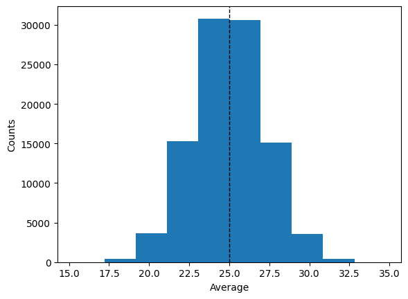
The mean (as expected) works very well to estimate the ‘mean’ of the population. What about the 2 definitions of variance?
plt.hist(variance_biased, bins=30)
plt.hist(variance_unbiased, bins=30, alpha=0.6)
plt.ylabel("Counts")
plt.axvline(S1**2, color="k", linestyle="dashed", linewidth=1)
plt.xlabel("Average")
plt.show()
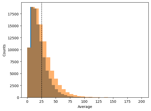
We see that the variance follows a \(\chi^2\) distribution. We can calculate the average values of these 2 distributions
print("The average value of the biased variance is", variance_biased.mean())
print("The average value of the unbiased variance is", variance_unbiased.mean())
The average value of the biased variance is 20.01855188790248
The average value of the unbiased variance is 25.023189859878098
Monte Carlo techniques allow us to study in detail given estimators characteristics and evaluate whether they are consistent, biased, and efficient.
Method of Moments (MoM)#
The method of moments involves equating sample moments with theoretical moments. So, let’s start by making sure we recall the definitions of theoretical moments, as well as learn the definitions of sample moments.
Definitions#
Theoretical moment: calculated from theoretical distributions
E(\(X^k\)) is the \(k^{th}\) (theoretical) moment of the distribution (about the origin), for \(k=1,2,3...\). This is given by E(\(X^k\))=\(\int_{-\infty}^\infty x^k f(x) dx\), where \(f(x)\) is the probability density distribution of our population.Sample moment: calculated from sampled data
\(M_k=\frac{1}{n}\sum_{i=1}^{n} x_i^k\) is the \(k^{th}\) sample moment for \(k=1,2,3...\)One Form of the Method
The basic idea behind this form of the method is to:Equate the first sample moment about the origin \(M_1=\frac{1}{n}\sum_{i=1}^{n} X_i\) to the first theoretical moment E(\(X\))
Equate the second sample moment about the origin \(M_2=\frac{1}{n}\sum_{i=1}^{n} X_i^2\) to the second theoretical moment E(\(X^2\))
Continue equating sample moments about the origin, \(M_k=\frac{1}{n}\sum_{i=1}^{n} X_i^k\) with the corresponding theoretical moments E(\(X^k\)) until you have as many equations as you have parameters.
Solve for the parameters.
The resulting values are called method of moments estimators. It seems reasonable that this method would provide good estimates, since the empirical distribution converges in some sense to the probability distribution. Therefore, the corresponding moments should be about equal.
Exercises#
Exercise 5
Let \(X_1, X_2, X_3... X_n\) be normal random variables with mean and variance. What are the method of moments estimators of the mean \(\mu\) and variance \(\sigma\)?
Solution to Exercise 5
Recall that
and
from this we have
and
Solving form \(\mu\) and \(\sigma\) we get that
and
which is the definition of variance
Exercise 6
The decay of a muon into a positron (\(e^+\)), an electron neutrino (\(\nu_e\)), and a muon antineutrino (\(\bar{\nu}_\mu\))
has a distribution angle \(t\) with density given by
where \(-\pi<t<\pi\), with \(t\) the angle between the positron trajectory and the \(\mu^+\)-spin. The anisometry parameter \(\alpha \in [1/3, 1/3]\) depends the polarization of the muon beam and positron energy. Based on the measurement \(t_1,...t_n\), give the method of moments estimate \(\hat{\alpha}\) for \(\alpha\). (Note: In this case the mean is 0 for all values of \(\alpha\), so we will have to compute the second moment to obtain an estimator.)
Solution to Exercise 6
The theoretical moment 1 is given by
so it doesnt provide any info. The theoretical moment 2 is given by
Equating the second sample moment \(M_2=\frac{1}{n}\sum_{i=1}^{n} t_i^2\) with the theoretical moment \(E(T^2)\) and solving for \(\alpha\) we get the MoM estimator \(\hat{\alpha}\)
The method of moments is fairly simple and yields consistent estimators (under very weak assumptions), though these estimators are often biased.
It is an alternative to the method of maximum likelihood. Due to easy computability, method-of-moments estimates may be used as the first approximation to the solutions of the likelihood equations!
Maximum Likelihood#
In statistics, maximum likelihood estimation (MLE) is a method of estimating the parameters of an assumed probability distribution, given some observed data.
This is achieved by maximizing a likelihood function so that, under the assumed statistical model, the observed data is most probable.
Let’s start with the Probability Density function (PDF) for the Normal distribution
Let’s say we take one sample from a population that follows this distribuition and our sample is 5. What is the probability it comes from a distribution of μ = 5 and σ = 3?
print("The probability is", norm.pdf(5, 5, 3))
The probability is 0.1329807601338109
What if it came from a distribution with μ = 7 and σ = 3?
print("The probability is", norm.pdf(5, 7, 3))
The probability is 0.10648266850745075
Consider this sample: x = [4, 5, 7, 8, 8, 9, 10, 5, 2, 3, 5, 4, 8, 9] and let’s compare these values to both PDF ~ N(5, 3) and PDF ~ N(7, 3). Our sample could be drawn from a variable that comes from these distributions, so let’s take a look.
Show code cell source
data = [4, 5, 7, 8, 8, 9, 10, 5, 2, 3, 5, 4, 8, 9]

x = np.linspace(0, 20, num=100)
plt.subplot(2, 1, 1)
plt.plot(x, stats.norm.pdf(x, 5, 3), label="N(5,3)")
plt.plot(x, stats.norm.pdf(x, 7, 3), label="N(7,3)")
plt.legend()
plt.subplot(2, 1, 2)
plt.hist(data, bins=20, range=(0, 20), label="data")
plt.legend()
plt.show()
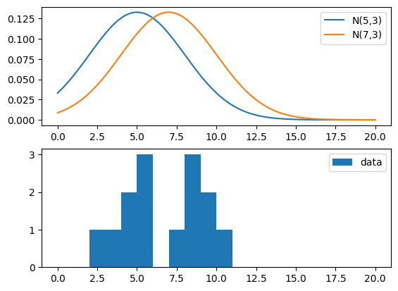
Which is the value of \(\mu\) and \(\sigma\) that most likely give rise to our data?
Definition#
Given a data sample \(X = \{x_1,x_2,\dots,x_N\}\) one applies an estimator \(\hat{a}\) for the quantity \(a\). The data values \(x_i\) are drawn from some probability density function \(P(x,a)\) which depends on \(a\). The form of \(P\) is given and \(a\) specified. The probability of a data set is the product of the individual probabilities.
This product is called likelihood.
The ML estimator for a parameter \(a\) is the procedure which evaluates the parameter value \(\hat{a}\) which makes the actual observations \(X\) as likely as possible, that is the set of parameters \(\hat{a}\) which maximises \(L(X;a)\). In practice, the logarithm of \(L\) is more practical to work with computationally (numerical stability):
The ML estimator \(\hat{a}\) is then the value of \(a\) which maximises \(\ln L(X;a)\) (or minimises \(-\ln L(X;a)\)). This can be found (in some cases analytically) by:
Why log? Simply because it helps with numerical stability, i.e. multiplying thousands of small values (probabilities, likelihoods, etc..) can cause an underflow in the system’s memory, and the log is a perfect solution because it transforms multiplications to additions and transforms small positive numbers into non-small negative numbers.
We now apply the definition of log(L) to the previous example. For simplicity we assume that \(\sigma=3\) is known. We will see later on more complex examples.
data = np.array([4, 5, 7, 8, 8, 9, 10, 5, 2, 3, 5, 4, 8, 9])
std = 3


@np.vectorize
def likelihood(mu) -> float:
    return np.sum(np.log(norm.pdf(data, mu, std)))
Show code cell source
mu = np.linspace(0, 12, num=100)
ll = likelihood(mu)

plt.plot(mu, ll, label="Likelihood")
plt.xlabel("mu")
plt.legend()
plt.show()
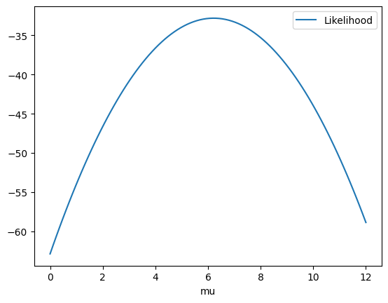
It is better to look for minima than for maxima so let’s put a - to the likelihood
@np.vectorize
def likelihood(mu) -> float:
    return -np.sum(np.log(norm.pdf(data, mu, std)))
So the routine found that the best value for mu is. actually 6.21 !!!
opt.fmin(func=likelihood, x0=1)
Optimization terminated successfully.
         Current function value: 32.821108
         Iterations: 21
         Function evaluations: 42
array([6.21425781])
(Even more) Examples#
Lifetime#
For decays with a lifetime \(\tau\), the (normalised) probability distribution as a function of time \(t\) is: \(P(t;\tau)=\frac{1}{\tau}\exp(-t/\tau)\). We calculate the function \(\ln L\) for this distribution in analytic way
Differentiating with respect to \(\tau\) and setting it to zero we obtain the estimator \(\hat{\tau}\) The maximum can be found as:
Discrete variable#
Suppose that \(X\) is a discrete random variable following the pdf
where \(0\le \theta \le1\).
First of all we check that the PDF is normalised
Suppose we have the following sequence : \((3,0,2,1,3,2,1,0,2,1)\). What is the value of \(\hat{\theta}\)?
We calculate \(\ln L\):
…. continue….
We need to calculate \(\frac{d \ln L}{d\theta}=0\) so all terms nodepending on \(\theta\) can be neglected.
Multiple dimensions#
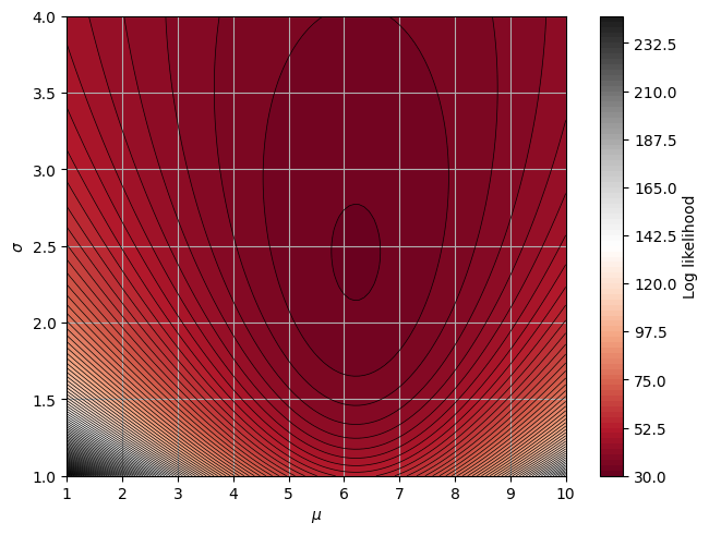
Let’s go back to the example involving the Gaussian PDF
Now assume that we want to esimtate both \(\mu\) and \(\sigma\) from a the same data set as we used before.
We define the loglikelihood function (with the - sign!)
@np.vectorize
def likelihood2(mu, sigma) -> float:
    return -np.sum(np.log(norm.pdf(data, mu, sigma)))
mu = np.linspace(1, 10, num=100)
sigma = np.linspace(1, 4, num=100)

a_grid, b_grid = np.meshgrid(mu, sigma)
Z = likelihood2(a_grid, b_grid)
Show code cell source
fig, ax = plt.subplots(constrained_layout=True)
levels = MaxNLocator(nbins=55).tick_values(Z.min(), Z.max())
n_levels = 100
plt.contour(a_grid, b_grid, Z, n_levels, linewidths=0.5, colors="k")
mesh = ax.contourf(a_grid, b_grid, Z, n_levels, cmap=plt.cm.RdGy)
cbar = fig.colorbar(mesh)
cbar.ax.set_ylabel("Log likelihood")

plt.ylabel(R"$\sigma$")
plt.xlabel(R"$\mu$")
ax.grid()
plt.show()
def optimizable_nll(params) -> float:
    mu, sigma = params
    return -np.sum(np.log(norm.pdf(data, mu, sigma)))
res = opt.minimize(optimizable_nll, x0=(6, 3))
res
  message: Optimization terminated successfully.
  success: True
   status: 0
      fun: 32.26919449213561
        x: [ 6.214e+00  2.425e+00]
      nit: 8
      jac: [-1.431e-06  4.768e-07]
 hess_inv: [[ 4.296e-01 -2.638e-03]
            [-2.638e-03  2.108e-01]]
     nfev: 33
     njev: 11
Properties of the ML estimator#
So how good are ML estimators?
Consistency: Usually, ML estimators are consistent. That is for increasing data sets, the estimator approaches the true value of the parameter.
Efficiency
Biaseness
Efficiency#
No such thing as a generally efficent estimator. Efficiency depends on the case considered.
Limit of Accuracy: Minimum Variance Bound (MVB)
For efficient estimators \(V(\hat{a})=MVB\)
For a Gaussian distribution:
What is the MVB?
The MVB for \(\mu\) is given by
The first derivative of \(LL\) with respct to \(\mu\) is just
and the second derivative
From this the standard error for the ML estimator of \(\mu\) is
Biaseness#
However, the ML estimator is often biased. This can be seen by calculating the likelihood function for a data set \(\{x_i\}\) with a common mean \(\mu\) and uncertainty \(\sigma\):
and find the maximum, where the partial derivatives are zero:
The ML estimator for the spread of a gaussian data set is \(\hat\sigma^2 = \frac{1}{N}\sum_i(x_i-\hat{\mu})^2\) which as we know is biased (does not include Bessel’s correction).
Uncertainty on ML estimators#
The uncertainty on a ML estimator can be found as discussed in relation to the efficiency:
for unbiased, efficient, ML estimators.
For several variables (\(N\)), the vector of estimated parameters \(\widehat{\vec{a}}\) is found by minimising the \(N\)-dimensional function \(-\ln\,L\). The inverse of the covariance matrix is then given by:
\(\mathrm{cov}^{-1}(a_i,a_j) = -\left.\frac{\partial^2\,\ln\,L}{\partial\,a_i\partial\,a_j}\right|_{\vec{a}=\widehat{\vec{a}}}\)
Inverse of the Hessian matrix.
There is some intuition in the plot above. The precision of the estimate \(\hat{a}\) can be measured by the curvature of the \(\ln L(a)\) function around its peak.
The easy way to think about this is to recognize that the curvature of the likelihood function tells us how certain we are about our estimate of our parameters. A flatter curve has more uncertainty. The second derivative of the likelihood function is a measure of the likelihood function’s curvature - this is why it provides our estimate of the uncertainty with which we have estimated our parameters.
Exercise 7
Show that the uncertainty of the estimator of \(\mu\) in the example above can be obtained by taking the difference between \(\hat{\mu}-\mu_1\), where \(\mu_1\) is the value of the parameter at the point where the log likelihood differs by 0.5 from its maximum point. \(\hat{\mu}\) is the value of \(\mu\) that maximises the log likelyhood.
Solution to Exercise 7
For the Gaussian PDF we have shown before that \(LL(\mu)=-\sum\frac{(x_i-\mu)^2}{2\sigma^2}-N\ln{\sigma\sqrt{2\pi}}\). From this, we get that
This can be rewritten as
Using the fact that \(\sum(x_i)=N\hat{\mu}\), we get
Therefore
which is consistend with the MVB.
MLE provides us with efficient and unbiased estimation when N is large. There is no loss of information through binning as all experimental information is used. It provides errors on its estimates. At small N, however, estimators CAN be biased. You need to make assumptions about the parent PDF and there is no way of estimating a “Goodness of fit”.
Fitting data – Method of least squares#
Introduction#
For a function \(f(x_i;a)\) and a data set \(\{x_i,y_i,\sigma_i\}\), assuming for each data point \(y_i\) is drawn from a Gaussian distribution of mean \(f(x_i;a)\) and spread \(\sigma_i\), we know that the likelihood function must obey:
The first part does not depent on our parameters.
Instead of minimising \(-\ln L\) we may therefore equivalently define and minimise:
I.e.\(\chi\)-squared minimisation, as you know it, is in fact the maximum-likelihood estimator of the function parameters \(a\)
This means that it comes with the nice properties of the ML estimator:
It is consistent (at least typically).
The bias is most often small.
It is efficient asymptotically (\(N\to\infty\)), and \(\pm1\sigma\) can be found by identifying where \(\chi^2\) changes by 1 from it’s minimum:
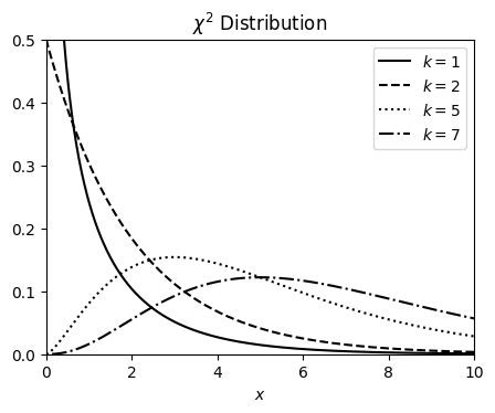
χ² PDF#
The \(\chi^2\) is a statistical distribution which is built as a sum of squares of \(k\)-gaussian (random) variables
Chi-square (\(\chi^2\)) distributions are a family of continuous probability distributions. They’re widely used in hypothesis tests, including the chi-square goodness of fit test and the chi-square test of independence.
The shape of a chi-square distribution is determined by the parameter k, which represents the degrees of freedom.
Very few real-world observations follow a chi-square distribution. The main purpose of chi-square distributions is hypothesis testing, not describing real-world distributions.
The corresponding PDF for the case of a continuous variable can be expressed as
We can calculate the mean \(\mu\) and the variance \(V\) and we get
# ------------------------------------------------------------
# Define the distribution parameters to be plotted
# We define 4 distributions with 4 different means
k_values = [1, 2, 5, 7]
linestyles = ["-", "--", ":", "-."]
mu = 0
x = np.linspace(-1, 20, num=1_000)
# ------------------------------------------------------------
Show code cell source
fig, ax = plt.subplots(figsize=(5, 3.75))
fig.subplots_adjust(bottom=0.12)
for k, ls in zip(k_values, linestyles):
    dist = chi2(k)
    res = plt.plot(x, dist.pdf(x), ls=ls, c="black", label=f"$k={k}$")
plt.xlim(0, 10)
plt.ylim(0, 0.5)
plt.xlabel("$x$")
plt.title(R"$\chi^2\ \mathrm{Distribution}$")
plt.legend()
plt.show()
Linear least squares#
Example: Fitting a straight line#
For a straight line fit to a data set \(\{x_i,y_i\}\) with common uncertainty \(\sigma\) we have \(f(x_i;m,c)=m\cdot x_i + c\), and:
We now differentiate and equate to zero as
and
Resolving the 2 equations we get
We thereby have established that \(\widehat{m}\) and \(\widehat{c}\) are linear in \(y_i\)
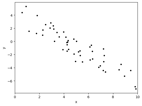
Covariance is a measure of the relationship between two random variables. The metric evaluates how much – to what extent – the variables change together (but not the strength of the relationship).
# Select a random seed so we can all generate the same sample
np.random.seed(123)
# Choose the "true" parameters.
m_true = -1
c_true = 4

# Generate some synthetic data from the model.
N = 50
x = np.sort(10 * np.random.rand(N))
y = m_true * x + c_true
y += np.random.randn(N)
plt.errorbar(x, y, fmt=".k", capsize=0)
starting_values = np.linspace(0, 10, num=500)
plt.xlim(0, 10)
plt.xlabel("x")
plt.ylabel("y")
plt.show()
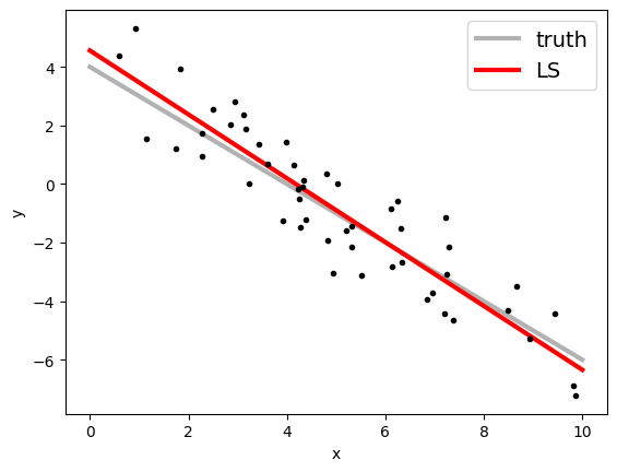
We apply the formulas:
xave = x.mean()
yave = y.mean()
cov = np.cov(x, y)[0][1]
var = np.cov(x, y)[0][0]

mfit = cov / var
cfit = yave - mfit * xave

print("Least-squares estimates:")
print("m = ", mfit)
print("c = ", cfit)
Least-squares estimates:
m =  -1.090298332414615
c =  4.5584490943071385
Show code cell source
plt.errorbar(x, y, fmt=".k", capsize=0)
plt.plot(
    starting_values,
    m_true * starting_values + c_true,
    "k",
    alpha=0.3,
    lw=3,
    label="truth",
)
plt.plot(starting_values, mfit * starting_values + cfit, "r", lw=3, label="LS")
plt.xlabel("x")
plt.ylabel("y")
plt.legend(fontsize=14)
plt.show()
Uncertainties and covariances for straight-line fit#
We can now calculate the errors on previous quantities by acting with derivatives over the ML.
We therefore get the inverse of the covariance matrix for \((m,c)\) to be:
By inverting the matrix we get
\(\sigma\) is the (common) uncertainty for the {\(y_i\)} measurements and \(V(x)\) is the variance in the {\(x_i\)} data. This means the variances (and covariance) in the fitted parameters \(c\) and \(m\) scales with the square of the uncertainty in {\(y_i\)}, as it should, and inversely with both \(N\) and \(V(x)\), such that a data set with many measurements and an extended measurement range has a reduced uncertainty (and variance) on the fitted parameters.
xave = x.mean()
xave2 = (x * x).mean()
var = np.cov(x, y)[0][0]
N = len(x)

Vcm = [[1, -xave], [-xave, xave2]]
Vcm = np.array(Vcm / (N * var))
Having access to the error matrix we can now read on the diagonal the error on m and c. While on the off diagonal we can read the correlation coefficiet
In statistics, the Pearson correlation coefficient (PCC) is a value that measures linear correlation between two sets of data. It is the ratio between the covariance of two variables and the product of their standard deviations; thus, it is essentially a normalized measurement of the covariance, such that the result always has a value between −1 and 1. As with covariance itself, the measure can only reflect a linear correlation of variables, and ignores many other types of relationships or correlations.
rho = Vcm[0][1] / (np.sqrt(Vcm[0][0] * Vcm[1][1]))

print("Least-squares estimates:")
print("m = ", mfit, "+/-", Vcm[0][0])
print("b = ", cfit, "+/-", Vcm[1][1])
print("rho=", rho)
Least-squares estimates:
m =  -1.090298332414615 +/- 0.00362663928191893
b =  4.5584490943071385 +/- 0.11094101522024427
rho= -0.90737508326441
Linear models#
In this section, we discuss models that are linear in parameter space, i.e. they can be written as
For example given the two functions
the function \(g(x,\mathbf{a})\) is not linear in its parameters!
We can write a linear model in a matrix form as
Here the function \(f\) has been evaluated over the \(x_N\) points that we use to fit the coupling constants.
The general form of \(\chi^2\) is
To obtain \(a_j\) we need to take the respective derivatives to them and set to 0 as standard MLE
if \(V_y\) is the (known) covariance matrix for the measured values of \(y\) (assuming no error on \(x\)), we can therefore express previous form in matrix form as
which gives the following \(\chi^2\) estimator (also ML estimator) of the parameter vector \(a\)
The \(M\)-matrix described above is used to calculate the covariance matrix for the estimator
Important remark on Unweighted Fitting
For an unweighted least-squares function, the covariance matrix should be multiplied by the variance of the residuals about the best-fit to give the variance-covariance matrix. This estimates the statistical error on the best-fit parameters from the scatter of the underlying data.
Non-linear model#
Consider the model \(f(x)=\sin(ax)\), where \(a\) is the parameter. If we fit on 5 data points. The number of degrees of freedom is 4.
We build some noisy data
def func(x, a):
    return np.sin(a * x)


np.random.seed(123)
n_points = 50
x = np.linspace(0, 20, num=n_points)
y = (np.sin(x / 3) + np.random.normal(np.sin(x / 3), 0.2)) / 2
y_error = np.random.normal(0.1, 0.02, size=n_points)
Show code cell source
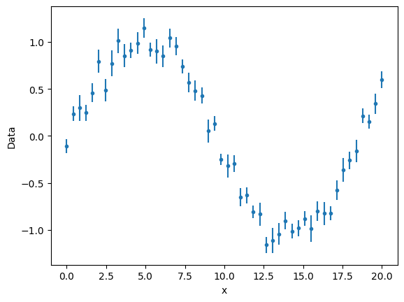
plt.errorbar(x, y, y_error, ls="", marker=".")
plt.xlabel("x")
plt.ylabel("Data")
plt.show()
gmodel = Model(func)
result = gmodel.fit(y, x=x, a=1)
result
Fit Result
Model: Model(func)
| fitting method | leastsq |
| # function evals | 119 |
| # data points | 50 |
| # variables | 1 |
| chi-square | 46.8836357 |
| reduced chi-square | 0.95680889 |
| Akaike info crit. | -1.21771545 |
| Bayesian info crit. | 0.69430756 |
| R-squared | -0.79068686 |
| name | value | standard error | relative error | initial value | min | max | vary |
|---|---|---|---|---|---|---|---|
| a | 1.04918825 | 0.01750715 | (1.67%) | 1 | -inf | inf | True |
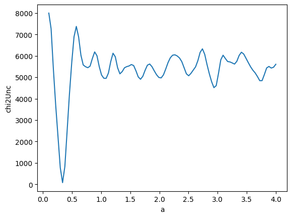
@np.vectorize
def chi2_uncertainty(a):
    z = func(x, a)
    return np.sum(((y - z) / y_error) ** 2)


av = np.linspace(0.1, 4, 100)
z = chi2_uncertainty(av)
Show code cell source
plt.plot(av, z, "-")
plt.xlabel("a")
plt.ylabel("chi2Unc")
plt.show()
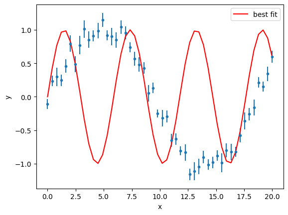
gmodel = Model(func)
result = gmodel.fit(y, a=1.2, x=x, weights=1 / y_error)
result
Fit Result
Model: Model(func)
| fitting method | leastsq |
| # function evals | 187 |
| # data points | 50 |
| # variables | 1 |
| chi-square | 4930.62050 |
| reduced chi-square | 100.624908 |
| Akaike info crit. | 231.559856 |
| Bayesian info crit. | 233.471879 |
| R-squared | -0.79475425 |
| name | value | standard error | relative error | initial value | min | max | vary |
|---|---|---|---|---|---|---|---|
| a | 1.06787231 | 0.01640931 | (1.54%) | 1.2 | -inf | inf | True |
Show code cell source
plt.errorbar(x, y, y_error, ls="", marker=".")
plt.plot(x, result.best_fit, "r-", label="best fit")
plt.legend(loc="best")
plt.xlabel("x")
plt.ylabel("y")
plt.show()
gmodel = Model(func)
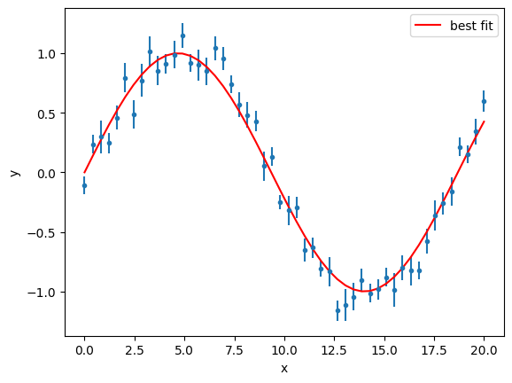
result = gmodel.fit(y, a=0.2, x=x, weights=1 / y_error)
result
Fit Result
Model: Model(func)
| fitting method | leastsq |
| # function evals | 15 |
| # data points | 50 |
| # variables | 1 |
| chi-square | 80.4941785 |
| reduced chi-square | 1.64273834 |
| Akaike info crit. | 25.8080930 |
| Bayesian info crit. | 27.7201160 |
| R-squared | 0.97387236 |
| name | value | standard error | relative error | initial value | min | max | vary |
|---|---|---|---|---|---|---|---|
| a | 0.33612704 | 0.00183776 | (0.55%) | 0.2 | -inf | inf | True |
Show code cell source
plt.errorbar(x, y, y_error, ls="", marker=".")
plt.plot(x, result.best_fit, "r-", label="best fit")
plt.legend(loc="best")
plt.xlabel("x")
plt.ylabel("y")
plt.show()
k = len(x) - 1
print("Number of degrees of freedom:", k)

r1 = np.sqrt(2 * chi2_uncertainty(a=1.41084859)) / np.sqrt(2 * k - 1)
r2 = np.sqrt(2 * chi2_uncertainty(a=0.33495704)) / np.sqrt(2 * k - 1)

print(r1, r2)
Number of degrees of freedom: 49
10.619600880257074 1.2938479735751014
Residuals#
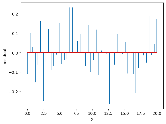
Residuals are the difference between the fitted model and the data.
Residuals are important when determining the quality of a model. You can examine residuals in terms of their magnitude and/or whether they form a pattern.
We use the previous example. We take the best fit and we calculate the residuals
Show code cell source
residual = y - result.best_fit
# plt.plot(x, residual, 'bo', label='Residuals')
fig, ax = plt.subplots()
ax.stem(x, residual, markerfmt=" ")
plt.xlabel("x")
plt.ylabel("residual")
plt.show()
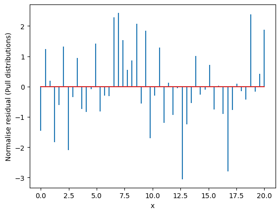
Show code cell source
residualUnc = (y - result.best_fit) / y_error
# plt.plot(x, residual, 'bo', label='Residuals')
fig, ax = plt.subplots()
ax.stem(x, residualUnc, markerfmt=" ")
plt.xlabel("x")
plt.ylabel("Normalise residual (Pull distributions)")
plt.show()
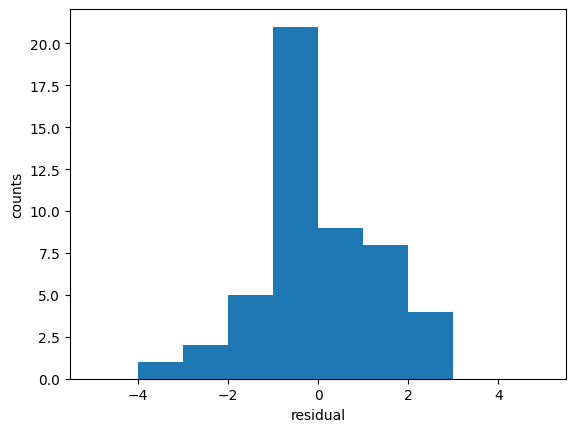
Show code cell source
counts, xbins, patches = plt.hist(residualUnc, bins=10, range=(-5, 5))
plt.xlabel("residual")
plt.ylabel("counts")
plt.show()
Show code cell source
# One can get the bin content and xvalues from the hist -- This would be necessary when one
# might want to fit the histogram

print(counts)
errcounts = []
for i in range(len(xbins) - 1):
    if counts[i] > 0:
        errcounts.append(np.sqrt(counts[i]))
    else:
        errcounts.append(10)
# Why do we do the above, i.e. setting zero values with large uncertainties?
xvals = []
for i in range(len(xbins) - 1):
    xvals.append((xbins[i] + xbins[i + 1]) / 2)
plt.errorbar(xvals, counts, errcounts, ls="", marker=".")
plt.xlabel("residual")
plt.ylabel("counts")
plt.show()
[ 0. 1. 2. 5. 21. 9. 8. 4. 0. 0.]
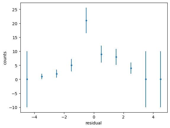
The residuals should be Gaussianly distributed with mean=0 and std=1. Deviations from this indicate issues with underfitting/overfitting/problems with uncertainties.
Where the average residual is not 0, it implies that the model is systematically biased (i.e., consistently over- or under-predicting).
Where residuals contain patterns, it implies that the model is qualitatively wrong, as it is failing to explain some property of the data. The existence of patterns invalidates most statistical tests.
Fitting Binned data: why a LSE might be biased here…#
Lets consider an example of measuring the lifetime of a particle using a PDF \(f(t;A, \tau)=A e^{t/\tau}\)
np.random.seed(32)

sample_size = 20
x = np.linspace(1, 10, num=sample_size)
y = np.vectorize(lambda z: np.random.poisson(13 * np.exp(-z / 3)))(x)
y
array([10,  6,  4,  9,  3,  3,  4,  2,  1,  0,  2,  2,  0,  1,  1,  0,  1,
        2,  0,  0])
data_x = x[y > 0]
data_y = y[y > 0]
data_y_err = np.sqrt(data_y)
# We generate noisy data on integer values of x to mimick the idea of bins and low-statistics...
plt.errorbar(data_x, data_y, data_y_err, ls="", marker=".")
# plt.plot(x,y,'o',label="data")
plt.xlabel("t")
plt.ylabel("counts")
plt.show()
Let’s start as usual with the \(\chi^2\) function exactly as we did before
def func(x, a, b):
    return a * np.exp(b * x)
gmodel = Model(func)
gmodel.nan_policy = "propagate"
result = gmodel.fit(data_y, x=data_x, weights=1 / data_y_err, a=12, b=-0.3)
result
Fit Result
Model: Model(func)
| fitting method | leastsq |
| # function evals | 22 |
| # data points | 15 |
| # variables | 2 |
| chi-square | 6.94946414 |
| reduced chi-square | 0.53457416 |
| Akaike info crit. | -7.54078469 |
| Bayesian info crit. | -6.12468429 |
| R-squared | 0.69079889 |
| name | value | standard error | relative error | initial value | min | max | vary |
|---|---|---|---|---|---|---|---|
| a | 10.2561191 | 2.27062248 | (22.14%) | 12 | -inf | inf | True |
| b | -0.33152914 | 0.06394921 | (19.29%) | -0.3 | -inf | inf | True |
| Parameter1 | Parameter 2 | Correlation |
|---|---|---|
| a | b | -0.8674 |
Show code cell source
plt.errorbar(data_x, data_y, data_y_err, ls="", marker=".")
plt.plot(data_x, result.best_fit, "-", label="Fit")
plt.legend()
plt.xlabel("t")
plt.ylabel("counts")
plt.show()
At this stage we just want to plot the \(\chi^2\) surface to see how it looks like. We can do a better analysis of the fit, but I leave it to you.
def chi2(a, b):
    return sum(
        ((y - func(x, a, b)) ** 2) / (ey**2)
        for x, y, ey in zip(data_x, data_y, data_y_err)
    )
grid_size = 500
a_grid, b_grid = np.meshgrid(
    np.linspace(0, 16, grid_size),
    np.linspace(-0.7, -0.15, grid_size),
)
Z = chi2(a_grid, b_grid)
fig, ax = plt.subplots(constrained_layout=True)
n_levels = 100
mesh = ax.contourf(a_grid, b_grid, Z, n_levels, cmap=plt.cm.PiYG)
plt.contour(a_grid, b_grid, Z, n_levels, linewidths=0.5, colors="k")
fig.colorbar(mesh)
plt.ylabel("-tau")
plt.xlabel("A")
ax.grid()
plt.show()
We have used here the standard \(\chi^2\) to perform the fit, but remeber this is based on the hypothesis that the underlying distribution is a Gaussian. What happens if we change the underlying distribution? What if instead of a Gaussian we use a Poisson, since here we are dealing with binned data and low-statistics?
Let’s now start again from the likelihood assuming a Poisson
or after some maths
The term \(+\ln y_i!\) does not depend on parameters so during minimisation we can forget it!
def like(param):
    a, b = param
    return sum(
        2 * (func(x, a, b) - y * np.log(func(x, a, b)))
        for x, y in zip(data_x, data_y)
    )
grid_size = 500
a_grid, b_grid = np.meshgrid(
    np.linspace(0, 16, grid_size),
    np.linspace(-0.7, -0.15, grid_size),
)
paramz = [a_grid, b_grid]
Z = like(paramz)
/tmp/ipykernel_2121/4144582212.py:4: RuntimeWarning: divide by zero encountered in log
  2 * (func(x, a, b) - y * np.log(func(x, a, b)))
Show code cell source
fig, ax = plt.subplots(constrained_layout=True)
n_levels = 100
mesh = ax.contourf(a_grid, b_grid, Z, n_levels, cmap=plt.cm.PiYG)
plt.contour(a_grid, b_grid, Z, n_levels, linewidths=0.5, colors="k")
fig.colorbar(mesh, ax=ax)
plt.ylabel("-tau")
plt.xlabel("$A$")
ax.grid()
plt.show()
p0 = [10, -0.3]
opt.fmin(like, p0, args=())
Optimization terminated successfully.
         Current function value: -43.738065
         Iterations: 31
         Function evaluations: 59
array([10.43504792, -0.28961542])
If you compare the results we get different values for A and \(\tau\) when the underlying distribution is Gaussian or a Poisson.
Show code cell source
plt.errorbar(data_x, data_y, data_y_err, ls="", marker=".")
plt.plot(data_x, result.best_fit, "-", label="Fit Gaussian")
plt.plot(data_x, func(data_x, 10.35008492, -0.26507234), "-", label="Fit Poisson")
plt.legend()
plt.xlabel("t")
plt.ylabel("counts")
plt.show()
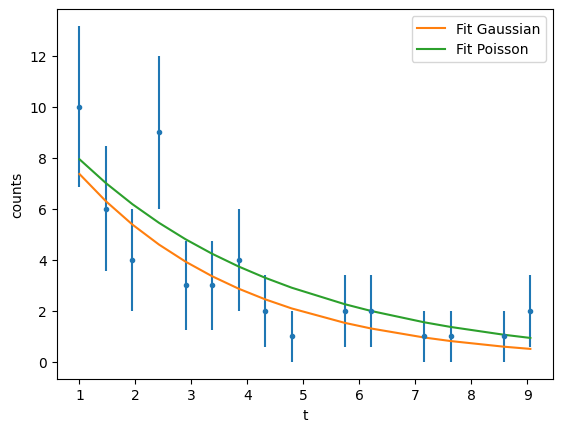
We see that the fit both reproduce “reasonably” the data but depending on which underlying distribution you assume you may get very different results!
Main exercise#
Exercise 8
The photoproduction of pions \(\gamma p \to p \pi^0\) using linearly polarised photons is associated with a probability function:
where A encompasses the overall normalisation, and \(\phi\) is the azimuthal distribution of the outgoing pion (the variable we measure in the laboratory), and takes values in the range from \(-\pi\) to \(\pi\). \(\Sigma\) is the observable of interest that we are asked to determine from a data se of measurements of \(\phi_i=[\phi_1,\phi_2,\phi_3,...,\phi_N]\)
[ ] Question 1
[ ] What are the three criteria we need to fulfill for the function above to be classified as a PDF? What is the value of A and the allaowed values of \(\Sigma\) for these criteria to be met?
[ ] Show that the MLE for \(\Sigma\) is
\[ \hat{\Sigma}=-\frac{\sum_i^N\cos(2\phi_i)}{\sum_i^N\cos^2(2\phi_i)} \](Hint: You can assume that \(\Sigma\) is small enough and apply the Taylor expansion \(\frac{1}{1-x}=1+x\))
[ ] Show that the MLE corresponds to a maximum point and show that the uncertainty of \(\hat{\Sigma}\) is
\[ \sigma_\Sigma=\frac{1}{\sqrt{\sum_i^N\cos^2(2\phi_i)}} \]
[ ] Question 2
[ ] Given the data in
Sigma.dat(these correspond to different measurements of \(\phi\) determine the \(\hat{\Sigma}\) and its uncertainty using your answers from part (a).[ ] Plot the \(\phi\) distribution of the data and discuss your choice of binning. Discuss the uncertainties associated with your yields (or counts) per bin and ensure these are illustrated in your plot.
[ ] Determine \(\Sigma\), its uncertainty, and the reduced \(\chi^2\) using a least squares fit. Discuss the values you obtained.
[ ] Plot the \(\chi^2\) surface.
Solution to Exercise 8
[x] Question 1
[x] The three criteria to fulfill for the differential cross section equation to be a PDF is single valued, positive, and normalised. For the cross section to be a PDF the values of \(\Sigma\) need to be between -1 and 1 so that the cross section is always a positive function. For the cross section function \(f(\phi,\Sigma)=\frac{d\sigma}{d\Omega}\) to be normalised we need to determined the constant A such that:
\[ \begin{equation} \int_{-\pi}^\pi f(\phi;A,\Sigma)d\phi=1. \end{equation} \]From this we have,
\[\begin{split} \begin{eqnarray} \int_{-\pi}^\pi f(\phi;A,\Sigma)d\phi&=&\int_{-\pi}^\pi A(1-\Sigma\cos(2\phi))d\phi \\ &=&\int_{-\pi}^\pi Ad\phi- A\Sigma\int_{-\pi}^\pi\cos(2\phi))d\phi\\ &=&A\phi{\large{|}}_{-\pi}^\pi-\frac{A\Sigma}{2}\sin(2\phi){\large{|}}_{-\pi}^\pi\\ &=&2\pi A, \end{eqnarray} \end{split}\]and thus \(A=\frac{1}{2\pi}\).
[x] For a given dataset with N entries we have the likelihood function:
and thus the loglikelihood
The MLE for \(\Sigma\) is determined by finding the value \(\hat{\Sigma}\) at which the \(LL\) is maximum, as:
Using the information tha \(\Sigma\) is small such that we can Taylor expand \(\frac{1}{1-\Sigma\cos(2\phi)}\) using \(\frac{1}{1-x}\approx1+x\), we get
and thus
[x] The \(LL\) is maximum when the second derivative is negative definite. The second derivative with respect to \(\Sigma\) is
which is always negative. The uncertainty in \(\hat{\Sigma}\), \(\sigma_{\Sigma}\) is then (using the MVB, which states \(V(\hat{x})=-\frac{1}{\frac{\partial^2 LL}{\partial x^2}}\))
[x] Question 2
[x] To calculate the MLE from the given dataset we need to open the file and loop over the entries to calculate the sums \(\sum_i^{N}\cos(2\phi_i)\) and \(\sum_i^{N}\cos^2(2\phi_i)\).
output_path = gdown.cached_download(
    url="https://drive.google.com/uc?id=1NUW8gsGoctzgRfeS3xTkLa10ySRIkMBV",
    path="data/Sigma.dat",
    md5="2b899234bb857efdd7129fc8c1d1aff3",
    quiet=True,
)
values = np.loadtxt(output_path)
sumcos2phi = np.sum(np.cos(2 * values))
sumcos2phiSqr = np.sum(np.cos(2 * values) * np.cos(2 * values))
est = -sumcos2phi / sumcos2phiSqr
print(f"Value of estimator: {est:.4f}")
unc = 1 / np.sqrt(sumcos2phiSqr)
print(f"Uncertainty of estimated value: {unc:.4f}")
/opt/hostedtoolcache/Python/3.10.14/x64/lib/python3.10/site-packages/gdown/cached_download.py:102: FutureWarning: md5 is deprecated in favor of hash. Please use hash='md5:xxx...' instead.
  warnings.warn(
Value of estimator: 0.1477
Uncertainty of estimated value: 0.0063
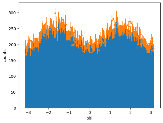
[x] We will be using mathplotlib errorsbars to plot the histogram of phi distributions. The uncertainties for each bin are determined using Poisson distribution since these are counting events: \(\sqrt{N_{bin}}\). We will first determine the number of bins we need and plot a histogram. From here, we can take the content of each bin to determine the uncertainty:
Show code cell source
bins = int(np.sqrt(len(values))) - 1
minim = min(values)
maxim = max(values)
print("Number of bins:", bins, " with bounds: ", minim, " and ", maxim)
binnedData, lowboundBin, patches = plt.hist(values, bins, range=(minim, maxim))
binnedUnc = []
xvalues = []
for i in range(len(binnedData)):
    binnedUnc.append(np.sqrt(binnedData[i]))
    xvalues.append((lowboundBin[i] + lowboundBin[i + 1]) / 2)
y = binnedData
x = xvalues
ery = binnedUnc
plt.errorbar(x, y, ery, ls="", marker=".")
plt.xlabel("phi")
plt.ylabel("counts")
plt.show()
Number of bins: 222 with bounds: -3.14157 and 3.14144
[x] For this, I will be using the lmfit routine that allows us to fit the distribution with an expression of the form \(Amp(1-\Sigma \cos(2\phi))\). Recall that the uncertainties here need to be passed appropriately by taking their reciprocal values.
recery = np.reciprocal(ery)
gmod = ExpressionModel("amp * (1-Sigma*cos(2*x))")
result = gmod.fit(y, x=x, amp=180, Sigma=-0.1, weights=recery)
print(result.fit_report())
[[Model]]
    <lmfit.ExpressionModel('amp * (1-Sigma*cos(2*x))')>
[[Fit Statistics]]
    # fitting method   = leastsq
    # function evals   = 10
    # data points      = 222
    # variables        = 2
    chi-square         = 177.798965
    reduced chi-square = 0.80817711
    Akaike info crit   = -45.2893019
    Bayesian info crit = -38.4839472
    R-squared          = 0.74815786
[[Variables]]
    amp:    224.423407 +/- 0.90387832 (0.40%) (init = 180)
    Sigma:  0.14729348 +/- 0.00564764 (3.83%) (init = -0.1)
Show code cell source
plt.errorbar(x, y, ery, ls="", marker=".")
plt.plot(x, result.init_fit, "--", label="initial fit")
plt.plot(x, result.best_fit, "-", label="best fit")
plt.xlabel("phi [rad]")
plt.ylabel("counts")
plt.legend()
plt.show()
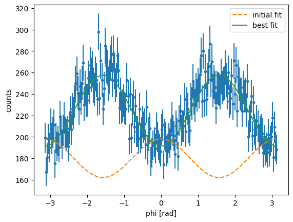
The obtained value for using least squares fitting \(\Sigma=0.147\pm0.006\), which is consistent with the MLE value. The reduced \(\chi^2\) is small, which indicates a good fit. It is worth noting here that the values obtained vary slightly with the choice of binning.
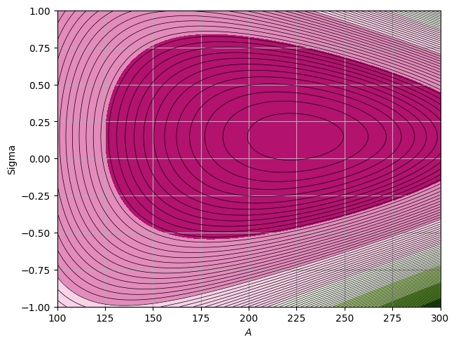
[x] For this we can create a function that calculates the \(\chi^2\) for any values of A and \(\Sigma\). We then create a grid of different values of \(A\) and \(\Sigma\) and plot the surface as follows:
def chi2(params):
    ll = 0
    Amp = params[0]
    Sigma = params[1]
    for i in range(len(x)):
        ll += ((y[i] - Amp * (1 - Sigma * np.cos(2 * x[i]))) ** 2) / ery[i] ** 2
    return ll
Show code cell source
Ax = np.linspace(100, 300, 500)
Bx = np.linspace(-1.0, 1.0, 500)

Axgrid, Bxgrid = np.meshgrid(Ax, Bx)
paramz = [Axgrid, Bxgrid]
Zgrid = chi2(paramz)
fig, ax = plt.subplots(constrained_layout=True)
levels = MaxNLocator(nbins=55).tick_values(Zgrid.min(), Zgrid.max())
cmap = plt.get_cmap("PiYG")
normB = BoundaryNorm(levels, ncolors=cmap.N, clip=True)
pc = ax.contourf(Axgrid, Bxgrid, Zgrid, cmap=cmap, norm=normB)
CS = plt.contour(Axgrid, Bxgrid, Zgrid, 100, linewidths=0.5, colors="k")

plt.ylabel("Sigma")
plt.xlabel("$A$")
ax.grid()
plt.show()
Extended Max Likelihood#
“This differs from the standard method of maximum likelihood in that the normalisation of the probability distribution function is allowed to vary. It is thus applicable to problems in which the number of samples obtained is itself a relevant measurement. If the function is such that its size and shape can be independently varied, then the estimates given by the extended method are identical to the standard maximum likelihood estimators, though the errors require care of interpretation. If the function does not have this property, then extended maximum likelihood can give better results.” Barlow https://doi.org/10.1016/0168-9002(90)91334-8
In conventional sampling theory an experiment usually consists of taking a predetermined number of samples.
In experimental physics, the collected number of events fluctuate following a Poisson distribution.
The number of events observed may be relevant to the quantities being estimated, and the incorporation of the fact that the number observed has the actual value \(\nu\) improves the estimates of the parameters \(\hat{\theta}\). To account for this, we “extend” the maximum likelihood by relaxing the normalisation of the PDF:
The likelihood function:
becomes
where \(n\sim Pois(n|\nu)\)
If \(\nu\) is independent of \(\theta\), the likelihood function becomes:
and the Log likelihood
The constant \(\ln n!\) does not depend on our observables, so it wont affect the maximum position and can thus be neglected.
To find the estimator for \(\nu\) we look for the minimum position in the negative loglikelihood:
which gives the maximum likelihood estimator \(\hat{\nu}=n\). The estimator for \(\theta\) results in the same estimator from our normal likelihood function
if \(\nu\) is dependent of \(\theta\) in the instance that \(\nu\) is a function of \(\theta\), \(\nu(\theta)\), then
and the resultand estimators exploit information from both \(n\) and \(x\), which will look to smaller variations in \(\hat{\theta}\).
(trivial) Example#
We are interested in determining the amount of events observed alongside with the characteristics of the PDF that describe our signal shape. Since the amount of signal collected follows a Poisson distribution, we can use the extended likelihood approach.
Lets first look at the data provided in ExtendedLLexample.txt:
output_path = gdown.cached_download(
    url="https://drive.google.com/uc?id=1p3kLa9XZAZXiLIszq7SxMmoiNZ_qLYXf",
    path="data/ExtendedLLexample.txt",
    md5="fcf1a7ff3bdeece6154d1fb1ca03ef97",
    quiet=True,
)
with open(output_path) as f:
    values = [float(line) for line in f.readlines()]
Show code cell source
bins = int(np.sqrt(len(values))) - 1
minim = min(values)
maxim = max(values)
print("Number of bins:", bins, " with bounds: ", minim, " and ", maxim)
binnedData, lowboundBin, patches = plt.hist(values, bins, range=(minim, maxim))
plt.show()
print("number of entries", len(values))
Number of bins: 21 with bounds: 1.07311 and 1.14384
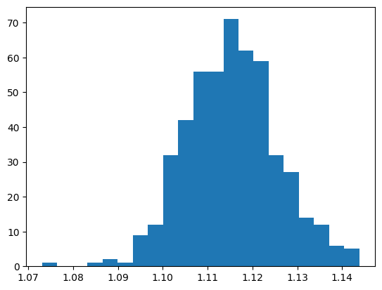
number of entries 500
From this our Signal seems to be described by a Gaussian function.
Using the equation from the previous slide the negative log likelihood is the given by:
def llog(params):
    s, mu, sigma = params
    return s - sum(np.log(s * norm.pdf(x, mu, sigma)) for x in values)
starting_values = [2000, 1.12, 0.01]
res = opt.minimize(llog, starting_values)
res
  message: Desired error not necessarily achieved due to precision loss.
  success: False
   status: 2
      fun: -4191.541854565566
        x: [ 5.001e+02  1.115e+00  1.018e-02]
      nit: 20
      jac: [-6.104e-05 -1.506e+00 -8.364e-01]
 hess_inv: [[ 3.021e+02 -9.169e-04 -7.067e-04]
            [-9.169e-04  2.216e-07  4.159e-09]
            [-7.067e-04  4.159e-09  1.109e-07]]
     nfev: 275
     njev: 66
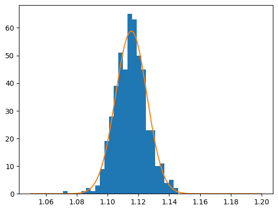
Using the extended maximum likelihood we get that the number of signal events is 500.
# We can plot the Gaussian function on top of our histogram. We need to scale the Gaussian function
# to our bin width to properly vizualise it.
x = np.linspace(1.05, 1.20, num=1_000)


def Gaus(x, params):
    s, mu, sigma = params
    Gausfun = s * norm.pdf(x, mu, sigma)
    return Gausfun * (1.2 - 1.05) / 50
Show code cell source
params = res.x
plt.hist(values, 50, range=(1.05, 1.2))
plt.plot(x, Gaus(x, params), "-", label="Fit Poisson")
plt.show()
This was a trivial example since one can also get the number of events from the entries. However, this approach can be very useful when we are dealing with signal and background contributions. In this case, we can use a two component fit, with a PDF that describes the background and a PDF that described our signal:
Normalised PDF:
where \(r=\frac{s}{s+b}\) is the ratio of signal to total. The prediction of the total number of events also follows a Poisson distribution with \(\nu=s+b\). From this we can write the negative log likelihood:
The extended ML method provides reliable values for obtained signal and background events and their corresponding uncertainties (Poisson fluctuations and uncertainty in proportion of signal to background)
Alternatively, one can also fit the normalised PDF:
and estimate the signal events by \(s=r\cdot n\). This however, does not provide us with reliable determination of uncertainties as \(\sigma_r\cdot n\) is not a good estimated of the variation of signal events as it ignores fluctuations in n.
Extended ML method is very useful when the determination of yield is needed – for example determination of cross section
Cross section describes the probability that two particles will collide and interact in a certain way, or for a specific reaction to occur. For example, the Rutherford cross-section is a measure of probability that an alpha particle will be deflected by a given angle during an interaction with an atomic nucleus.
When a cross section is specified as the differential limit of a function of some final-state variable, such as particle angle or energy, it is called a differential cross section. When a cross section is integrated over all scattering angles (and possibly other variables), it is called a total cross section or integrated total cross section
The probability that a reaction takes places can be written as:
where \(Y\) denotes the Yield of produced events and \(L\) denotes the luminosity.
The luminosity \(L\) is a measure of the colliding frequency between beam and target, and thus accounts for characteristics of the initial state of the reaction. Specifically, (for a fixed target experiments) the luminosity is proportional to the number of target centers and the incident number of beam particles. Lets take as an example the photoproduction of single pions \(\gamma p \to p \pi^0\). Here the luminosity is:
where \(\Phi\) is the number of photons incident on the target, \(\rho\) is the target density, \(l\) is the target length, \(A_r\) is the atomic weight of the target, and \(N_A\) is Avocadrons number.
(Note: Things can get more complicated in collider experiments. See https://cds.cern.ch/record/941318/files/p361.pdf for a summary on luminosity determination).
The yield of produced events \(Y\) can be determined in experiments by identifying the final state particles of the reaction (using for example detectors). In this approach, one needs to acount for limitations in the detector acceptance (detector blind spots) and detector efficiency:
where \(Y_{det}\) is the number of events for our reaction of interest that were detected in our system, \(A\) is the detector acceptance, and \(epsilon\) is the detector efficiency. The denominator, here which is a correction factor for the detected yields can be established using sophistigated Monte Carlo approaches, and realistic detector simulations. This approach also allows us to account for inefficiencies in our analysis resulting in lost events in addition to detector inneficiencies.