Lecture 12 – Longitudinal plot#
Prepare the notebook with the preambles for the inclusion of pandas, numpy and matplotlib.pyplot. Import the data file (csv format) into Google Colab through the drive.mount command, import the pylorentz package.
Import Python libraries
import matplotlib.pyplot as plt
import numpy as np
import pandas as pd
from pylorentz import Momentum4
import gdown

output_path = gdown.cached_download(
    url="https://drive.google.com/uc?id=1VkG1gYY4qnfqNz3MEUkOKDwcAW4EF4uR",
    path="data/gammapi_2pions_exclusivityCuts.dat",
    md5="6aa2ab1388aa7fc1ce0568e3e972e491",
    quiet=True,
)
data = pd.read_csv(output_path)
data.columns = data.columns.str.strip()
data
/opt/hostedtoolcache/Python/3.10.14/x64/lib/python3.10/site-packages/gdown/cached_download.py:102: FutureWarning: md5 is deprecated in favor of hash. Please use hash='md5:xxx...' instead.
  warnings.warn(
| p1x | p1y | p1z | E1 | p2x | p2y | p2z | E2 | p3x | p3y | p3z | E3 | pgamma | helGamma | ||
|---|---|---|---|---|---|---|---|---|---|---|---|---|---|---|---|
| 0 | 0.517085 | 0.161989 | 0.731173 | 0.920732 | -0.254367 | 0.082889 | 0.495509 | 0.580189 | -0.259266 | -0.265152 | 0.445175 | 1.10275 | 1.657800 | -1 | |
| 1 | -0.216852 | -0.245333 | 0.107538 | 0.371878 | -0.183380 | 0.191897 | 0.145128 | 0.333213 | 0.389750 | 0.112110 | 0.790133 | 1.29195 | 1.044790 | -1 | |
| 2 | 0.197931 | 0.071432 | -0.010077 | 0.252778 | -0.111780 | -0.360482 | 0.367842 | 0.545221 | -0.090228 | 0.302313 | 0.724911 | 1.22694 | 1.095470 | -1 | |
| 3 | -0.505371 | -0.163949 | 0.450407 | 0.710395 | -0.141057 | 0.282404 | 1.186530 | 1.235730 | 0.679497 | -0.112014 | 0.729706 | 1.37371 | 2.388690 | -1 | |
| 4 | -0.200253 | -0.221165 | 0.289284 | 0.438425 | -0.160384 | 0.203285 | 0.051361 | 0.298667 | 0.350804 | -0.023423 | 0.645083 | 1.19168 | 0.998451 | -1 | |
| ... | ... | ... | ... | ... | ... | ... | ... | ... | ... | ... | ... | ... | ... | ... | ... |
| 433577 | -0.178174 | -0.006874 | 0.109490 | 0.251590 | -0.050105 | -0.335385 | 0.117234 | 0.385037 | 0.168768 | 0.324913 | 0.765021 | 1.26478 | 0.954648 | 1 | |
| 433578 | 0.280767 | -0.090755 | 0.280987 | 0.430740 | -0.192089 | -0.213071 | 0.090846 | 0.331763 | -0.047556 | 0.315046 | 0.640514 | 1.17988 | 1.003180 | -1 | |
| 433579 | 0.128575 | -0.018500 | 0.143663 | 0.238807 | 0.378718 | -0.051974 | 0.461311 | 0.615185 | -0.497148 | 0.087386 | 0.483961 | 1.17020 | 1.083930 | -1 | |
| 433580 | -0.262395 | -0.235015 | 0.024120 | 0.379712 | 0.330904 | -0.040001 | 0.751630 | 0.834003 | -0.095422 | 0.256882 | 0.695036 | 1.19938 | 1.492470 | 1 | |
| 433581 | -0.068621 | 0.111528 | -0.032843 | 0.194273 | -0.274412 | -0.101159 | 0.115541 | 0.344094 | 0.325894 | -0.006340 | 0.781223 | 1.26369 | 0.862625 | -1 |
433582 rows × 15 columns
Let’s prepare the relevant arrays containing the 4-momenta kinematics of the three particle (plus the two in the intial state), both in the laboratory and in the center of mass reference systems:
# final state
pip = Momentum4(data.E1, data.p1x, data.p1y, data.p1z)
pim = Momentum4(data.E2, data.p2x, data.p2y, data.p2z)
proton = Momentum4(data.E3, data.p3x, data.p3y, data.p3z)

# initial state
n_events = len(data)
zeros = np.zeros(n_events)
ones = np.ones(n_events)
m_proton = 0.93827
gamma = Momentum4(data.pgamma, zeros, zeros, data.pgamma)
target = Momentum4(m_proton * ones, zeros, zeros, zeros)
# 4-momenta in the scenter of mass system
cm = gamma + target
pip_cm = pip.boost_particle(-cm)
pim_cm = pim.boost_particle(-cm)
proton_cm = proton.boost_particle(-cm)
gamma_cm = gamma.boost_particle(-cm)
target_cm = target.boost_particle(-cm)
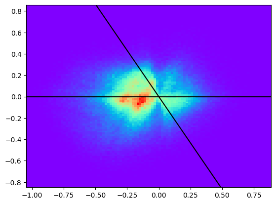
A longitudinal plot (introduced for the first time by Van Hove in 1969) offers a way to separate the contribution of different reaction production mechanisms. Inspecting a longitudinal plot may suggest particular selections in the longitudinal phase space which can help selecting specific reaction channels, enhancing for instance the contribution of meson versus baryon resonances. They are based on the assumption that at sufficiently high center-of-mass energies the phase space is reflected mainly by the longitudinal components of the particle momenta, while the transverse components can be neglected. Longitudinal plots are a convenient way to visualize the reaction kinematics of a reaction with three particles in the final state, in the form of 2D scattering plots (for \(n\) particles in the final state, the reaction kinematics are visualized in a \((n-1)\) dimensional plane). For a reaction with a three particles final state one defines a set of polar coordinates \(q\) and \(\omega\) such that, being \(q_1,\; q_2,\; q_3\) the longitudinal momentum components of each of them:
In a longitudinal plot the \((X,Y)\) coordinates are defined as follows:
Let’s build the cartesian coordinates arrays and make the scatter plot.
q1 = pip_cm.p_z
q2 = pim_cm.p_z
q3 = proton_cm.p_z
q = np.sqrt(q1**2 + q2**2 + q3**2)
a = np.sqrt(3 / 2) * q1 / q
filter_ = np.abs(a) <= 1
sin_omega = a[filter_]
cos_omega = (2 * q2 + q1) / np.sqrt(2) / q
cos_omega = cos_omega[filter_]
omega = np.arcsin(sin_omega)
omega = np.select(
    [(cos_omega < 0) & (sin_omega >= 0), True],
    [np.pi - omega, omega - np.pi],
)
X = q[filter_] * cos_omega
Y = q[filter_] * sin_omega
Show code cell source
plt.hist2d(X, Y, bins=100, cmap="rainbow")
plt.plot([-10, 10], [0, 0], color="black")
sixty = np.pi / 3
plt.plot(
    [-10 * np.cos(sixty), 10 * np.cos(sixty)],
    [10 * np.sin(sixty), -10 * np.sin(sixty)],
    color="black",
)
plt.plot(
    x3=[10 * np.cos(sixty), -10 * np.cos(sixty)],
    y3=[10 * np.sin(sixty), -10 * np.sin(sixty)],
    color="black",
)
plt.show()
Try with another input file (see here on Google Drive, for instance the generated MonteCarlo events at 5 or 10 GeV incident momentum) and check the differences. The whole folder can be downloaded as follows:
gdown.download_folder(id="1-Knh70_vLuctCkcg9oIIIIBaX2EPYkea", output="data", quiet=True)
Then set data to for instance
data = pd.read_csv("data/FurtherFun/gammaP_5GeV_protKPlusKMinusEtamiss.csv")
and rerun the notebook.