Lecture 12 – Phase space simulation#
How to perform a phase space simulation with Python?
Prepare the notebook by importing numpy, matplotlib.pyplot, and pylorentz and download the data file (CSV format) from Google Drive.
Import Python libraries
import matplotlib.pyplot as plt
import numpy as np
import phasespace
import tensorflow as tf
from pylorentz import Momentum4
Two-body decay#
Let’s start with a simple two body decay at rest: \(B^0\rightarrow K^+\pi^-\).
B0_MASS = 5279.65
PION_MASS = 139.57018
KAON_MASS = 493.677
n_events = 100_000

decay = phasespace.nbody_decay(B0_MASS, [PION_MASS, KAON_MASS])
weights, four_momenta = decay.generate(n_events=n_events)
WARNING: All log messages before absl::InitializeLog() is called are written to STDERR
I0000 00:00:1723042687.464384    2332 service.cc:146] XLA service 0x7fcf30006450 initialized for platform Host (this does not guarantee that XLA will be used). Devices:
I0000 00:00:1723042687.465023    2332 service.cc:154]   StreamExecutor device (0): Host, Default Version
I0000 00:00:1723042687.488908    2334 device_compiler.h:188] Compiled cluster using XLA!  This line is logged at most once for the lifetime of the process.
The simulation produces a dictionary (four_momenta) of tf.Tensor objects. Each object can be addressed with particles['p_i'], where i is the number of the \(i\)-th generated particle.
four_momenta
{'p_0': <tf.Tensor: shape=(100000, 4), dtype=float64, numpy=
 array([[ -826.70509119,  1913.87066299, -1578.34925398,  2618.58901417],
        [ 1900.11299646, -1207.10507879,  1330.41216148,  2618.58901417],
        [ 1758.49048017,   392.47454118, -1895.04711173,  2618.58901417],
        ...,
        [ 1017.00593996,  1059.02644352, -2163.72144695,  2618.58901417],
        [  790.0485493 ,  1548.24243445, -1953.5345515 ,  2618.58901417],
        [-2119.82949482,   146.14489215, -1523.97282566,  2618.58901417]])>,
 'p_1': <tf.Tensor: shape=(100000, 4), dtype=float64, numpy=
 array([[  826.70509119, -1913.87066299,  1578.34925398,  2661.06098583],
        [-1900.11299646,  1207.10507879, -1330.41216148,  2661.06098583],
        [-1758.49048017,  -392.47454118,  1895.04711173,  2661.06098583],
        ...,
        [-1017.00593996, -1059.02644352,  2163.72144695,  2661.06098583],
        [ -790.0485493 , -1548.24243445,  1953.5345515 ,  2661.06098583],
        [ 2119.82949482,  -146.14489215,  1523.97282566,  2661.06098583]])>}
Each tf.Tensor can be converted to a NumPy array, which can then be converted to a pylorentz.
def to_lorentz(p: tf.Tensor) -> Momentum4:
    p = p.numpy().T
    return Momentum4(p[3], *p[:3])
pion = to_lorentz(four_momenta["p_0"])
kaon = to_lorentz(four_momenta["p_1"])
These objects can be used to do kinematic computations. Let’s first verify that the invariant mass of the kaon+pion system corresponds to the mass of the mother \(B^0\):
B0 = pion + kaon
np.testing.assert_almost_equal(B0.m.mean(), B0_MASS)
Let’s also plot the momentum components of the two daugther particles.
Show code cell source
fig, ax = plt.subplots(1, 4, tight_layout=True, figsize=(11, 3.5))
ax[0].hist(B0.m, bins=100, color="CornFlowerBlue", range=(5279, 5280))
ax[0].set_xlabel(R"i.m.($\pi$K) [MeV/$c^2$]")
ax[0].set_title("(pion-kaon) i.m. \n")

ax[1].hist(kaon.p_x, bins=70, color="lightcoral", hatch="//")
ax[1].hist(
    pion.p_x,
    bins=70,
    color="springgreen",
    histtype="barstacked",
    hatch="\\",
    alpha=0.5,
)
ax[1].set_xlabel("$p_x$ [MeV/$c$]")
ax[1].set_title("x mom. component \n")

ax[2].hist(kaon.p_y, bins=70, color="lightcoral", hatch="//")
ax[2].hist(
    pion.p_y,
    bins=70,
    color="springgreen",
    histtype="barstacked",
    hatch="\\",
    alpha=0.5,
)
ax[2].set_xlabel("$p_y$ [MeV/$c$]")
ax[2].set_title("y mom. component \n")

ax[3].hist(kaon.p_z, bins=70, color="lightcoral", hatch="//")
ax[3].hist(
    pion.p_z,
    bins=70,
    color="springgreen",
    histtype="barstacked",
    hatch="\\",
    alpha=0.5,
)
ax[3].set_xlabel("$p_z$ [MeV/$c$]")
ax[3].set_title("z mom. component \n")
plt.show()
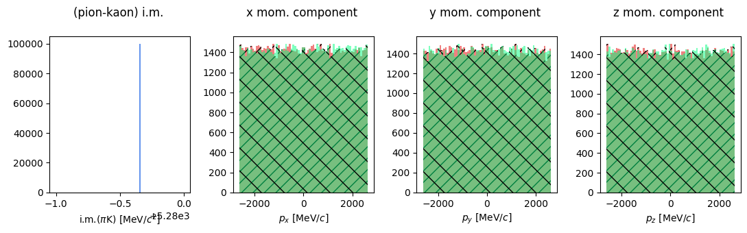
But it’s monochromatic!! of course it is… it’s a decay at rest. The momentum components are uniformly distributed in the available phase space.
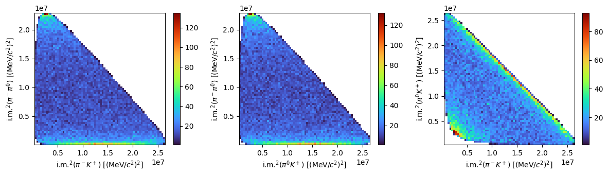
Three-body decay#
Let’s consider now a three body decay like \(B^0\rightarrow K^+\pi^-\pi^0\) and repeat the plot of the relevant kinematic variables. We can also make Dalitz plots this time.
n_events = 50_000
PION0_MASS = 134.9766
decay = phasespace.nbody_decay(B0_MASS, [PION_MASS, PION0_MASS, KAON_MASS])
weights, four_momenta = decay.generate(n_events=n_events)
pim = to_lorentz(four_momenta["p_0"])
pi0 = to_lorentz(four_momenta["p_1"])
kaon = to_lorentz(four_momenta["p_2"])
s1 = (kaon + pim).m2
s2 = (kaon + pi0).m2
s3 = (pim + pi0).m2
Show code cell source
fig, ax = plt.subplots(1, 3, tight_layout=True, figsize=(12, 3.5))
f0 = ax[0].hist2d(s1, s3, bins=70, cmap="turbo", cmin=1)
fig.colorbar(f0[3], ax=ax[0])
ax[0].set_xlabel(R"i.m.$^2(\pi^-K^+)$ [(MeV/$c^2)^2]$")
ax[0].set_ylabel(R"i.m.$^2(\pi^-\pi^0)$ [(MeV/$c^2)^2]$")

f1 = ax[1].hist2d(s2, s3, bins=70, cmap="turbo", cmin=1)
fig.colorbar(f1[3], ax=ax[1])
ax[1].set_xlabel(R"i.m.$^2(\pi^0K^+)$ [(MeV/$c^2)^2]$")
ax[1].set_ylabel(R"i.m.$^2(\pi^-\pi^0)$ [(MeV/$c^2)^2]$")

f2 = ax[2].hist2d(s1, s2, bins=70, cmap="turbo", cmin=1)
fig.colorbar(f2[3], ax=ax[2])
ax[2].set_xlabel(R"i.m.$^2(\pi^-K^+)$ [(MeV/$c^2)^2]$")
ax[2].set_ylabel(R"i.m.$^2(\pi^0K^+)$ [(MeV/$c^2)^2]$")
plt.show()
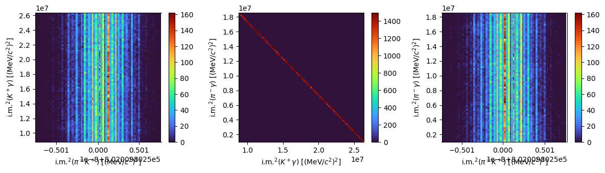
Decay chain#
The phasespace package allows to treat also multiple decays. Let’s consider the \(B^0\rightarrow K^{\ast 0}\gamma\) decay, followed by \(K^{\ast 0}\rightarrow \pi^-K^+\). It can be simulated using the following procedure:
from phasespace import GenParticle

B0_MASS = 5279.65
K0STAR_MASS = 895.55
PION_MASS = 139.57018
KAON_MASS = 493.677
GAMMA_MASS = 0.0

Kp = GenParticle("K+", KAON_MASS)
pim = GenParticle("pi-", PION_MASS)
Kstar = GenParticle("KStar", K0STAR_MASS).set_children(Kp, pim)
gamma = GenParticle("gamma", GAMMA_MASS)
B0 = GenParticle("B0", B0_MASS).set_children(Kstar, gamma)

weights, four_momenta = B0.generate(n_events=100_000)
four_momenta
{'KStar': <tf.Tensor: shape=(100000, 4), dtype=float64, numpy=
 array([[-2005.9755242 ,   818.79981645,  1370.79138976,  2715.77793272],
        [ -259.38770112,  1966.47210557, -1624.54469187,  2715.77793272],
        [ 1832.41089811,   999.44389302, -1488.89965497,  2715.77793272],
        ...,
        [ 1371.326898  ,  1909.74706848,  1022.62830521,  2715.77793272],
        [-2546.43612216,   293.99088437,    51.69538687,  2715.77793272],
        [-2164.06558774,  1214.27298959,  -644.82650076,  2715.77793272]])>,
 'gamma': <tf.Tensor: shape=(100000, 4), dtype=float64, numpy=
 array([[ 2005.9755242 ,  -818.79981645, -1370.79138976,  2563.87206728],
        [  259.38770112, -1966.47210557,  1624.54469187,  2563.87206728],
        [-1832.41089811,  -999.44389302,  1488.89965497,  2563.87206728],
        ...,
        [-1371.326898  , -1909.74706848, -1022.62830521,  2563.87206728],
        [ 2546.43612216,  -293.99088437,   -51.69538687,  2563.87206728],
        [ 2164.06558774, -1214.27298959,   644.82650076,  2563.87206728]])>,
 'K+': <tf.Tensor: shape=(100000, 4), dtype=float64, numpy=
 array([[ -768.92879359,   139.51993406,   594.82216053,  1099.20320442],
        [  135.81353503,  1086.77046943,  -867.52474327,  1481.83384023],
        [ 1337.40467274,   969.18525154,  -942.07436807,  1964.48273236],
        ...,
        [ 1314.08785087,  1589.58411581,  1038.88476312,  2361.48323568],
        [-1400.31563145,   -39.2651549 ,   222.83919804,  1501.93205857],
        [-1211.20701008,  1000.01745834,  -484.60855362,  1716.28079545]])>,
 'pi-': <tf.Tensor: shape=(100000, 4), dtype=float64, numpy=
 array([[-1237.04673061,   679.27988239,   775.96922923,  1616.5747283 ],
        [ -395.20123615,   879.70163614,  -757.0199486 ,  1233.9440925 ],
        [  495.00622537,    30.25864148,  -546.82528691,   751.29520036],
        ...,
        [   57.23904713,   320.16295267,   -16.25645792,   354.29469704],
        [-1146.12049072,   333.25603926,  -171.14381116,  1213.84587415],
        [ -952.85857765,   214.25553124,  -160.21794714,   999.49713727]])>}
gamma = to_lorentz(four_momenta["gamma"])
pion = to_lorentz(four_momenta["pi-"])
kaon = to_lorentz(four_momenta["K+"])
Kstar = to_lorentz(four_momenta["KStar"])
Let’s build the Dalitz plots matching particle pairs. The particles measured in the final state are \(K^-,\; \pi^-\) and \(\gamma\).
s1 = (pion + kaon).m2
s2 = (gamma + kaon).m2
s3 = (gamma + pion).m2
Show code cell source
fig, ax = plt.subplots(1, 3, tight_layout=True, figsize=(12, 3.5))

f0 = ax[0].hist2d(s1, s2, bins=70, cmap="turbo")
fig.colorbar(f0[3], ax=ax[0])
ax[0].set_xlabel(R"i.m.$^2(\pi^-K^+)$ [(MeV/$c^2)^2]$")
ax[0].set_ylabel(R"i.m.$^2(K^+\gamma)$ [(MeV/$c^2)^2]$")

f1 = ax[1].hist2d(s2, s3, bins=70, cmap="turbo")
fig.colorbar(f1[3], ax=ax[1])
ax[1].set_xlabel(R"i.m.$^2(K^+\gamma)$ [(MeV/$c^2)^2]$")
ax[1].set_ylabel(R"i.m.$^2(\pi^-\gamma)$ [(MeV/$c^2)^2]$")

f2 = ax[2].hist2d(s1, s3, bins=70, cmap="turbo")
fig.colorbar(f2[3], ax=ax[2])
ax[2].set_xlabel(R"i.m.$^2(\pi^-K^+)$ [(MeV/$c^2)^2]$")
ax[2].set_ylabel(R"i.m.$^2(\pi^-\gamma)$ [(MeV/$c^2)^2]$")
plt.show()
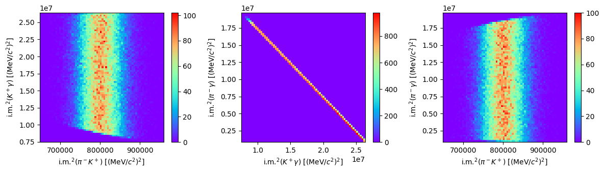
Width distribution#
These distributions aren’t so interesting, because the masses of each particle are one fixed value. So let’s simulate a more realistic \(K^\ast\) particle; not monochromatic, but with a width of 47 MeV.[1] The mass is extracted from a Gaussian distribution centered at the B0_MASS value and with \(\sigma = 47/2.36 \sim 20\) MeV. See more info on how to do this with the phasespace package here.
import tensorflow as tf
import tensorflow_probability as tfp

K0STAR_WIDTH = 47 / 2.36


def kstar_mass(min_mass, max_mass, n_events):
    min_mass = tf.cast(min_mass, tf.float64)
    max_mass = tf.cast(max_mass, tf.float64)
    kstar_mass_cast = tf.cast(K0STAR_MASS, dtype=tf.float64)
    tf.cast(K0STAR_WIDTH, tf.float64)
    tf.broadcast_to(kstar_mass_cast, shape=(n_events,))
    return tfp.distributions.TruncatedNormal(
        loc=K0STAR_MASS,
        scale=K0STAR_WIDTH,
        low=min_mass,
        high=max_mass,
    ).sample()
K = GenParticle("K+", KAON_MASS)
pion = GenParticle("pi-", PION_MASS)
Kstar = GenParticle("KStar", kstar_mass).set_children(K, pion)
gamma = GenParticle("gamma", GAMMA_MASS)
B0 = GenParticle("B0", B0_MASS).set_children(Kstar, gamma)
weights, four_momenta = B0.generate(n_events=100_000)
gamma = to_lorentz(four_momenta["gamma"])
pion = to_lorentz(four_momenta["pi-"])
kaon = to_lorentz(four_momenta["K+"])
Kstar = to_lorentz(four_momenta["KStar"])
Now you have all the 4-vectors to plot the invariant mass distributions for the different steps of the decay chains.
s1 = (pion + kaon).m2
s2 = (gamma + kaon).m2
s3 = (gamma + pion).m2
Show code cell source
fig, ax = plt.subplots(1, 3, tight_layout=True, figsize=(12, 3.5))
f0 = ax[0].hist2d(s1, s2, bins=70, cmap="rainbow")
fig.colorbar(f0[3], ax=ax[0])
ax[0].set_xlabel(R"i.m.$^2(\pi^-K^+)$ [(MeV/$c^2)^2]$")
ax[0].set_ylabel(R"i.m.$^2(K^+\gamma)$ [(MeV/$c^2)^2]$")

f1 = ax[1].hist2d(s2, s3, bins=70, cmap="rainbow")
fig.colorbar(f1[3], ax=ax[1])
ax[1].set_xlabel(R"i.m.$^2(K^+\gamma)$ [(MeV/$c^2)^2]$")
ax[1].set_ylabel(R"i.m.$^2(\pi^-\gamma)$ [(MeV/$c^2)^2]$")

f2 = ax[2].hist2d(s1, s3, bins=70, cmap="rainbow")
fig.colorbar(f2[3], ax=ax[2])
ax[2].set_xlabel(R"i.m.$^2(\pi^-K^+)$ [(MeV/$c^2)^2]$")
ax[2].set_ylabel(R"i.m.$^2(\pi^-\gamma)$ [(MeV/$c^2)^2]$")
plt.show()