Lecture 24 – Maximum Likelihood

Lecture 24 – Maximum Likelihood#

First we need to mount your drive directory and load some dependencies. Make sure your google drive system is configured

go to Shared with me directory
Right click on “Colab - Exp Meth. Hadron Spec “ //note extra space at end
right click and go to “organise” then “add shortcut”
add shortcut to My Drive

We will now be able to access this directory in our Colab notebook from /content/drive/MyDrive/Colab - Exp Meth. Hadron Spec /

Now run the next cell to actually mount the drive. Note you will need to give permissions for Colab to access your google account.

Load some helper functions from another notebook lecture24_utilities.ipynb by running the following cell.

Dealing with backgrounds#

Toy Dataset#

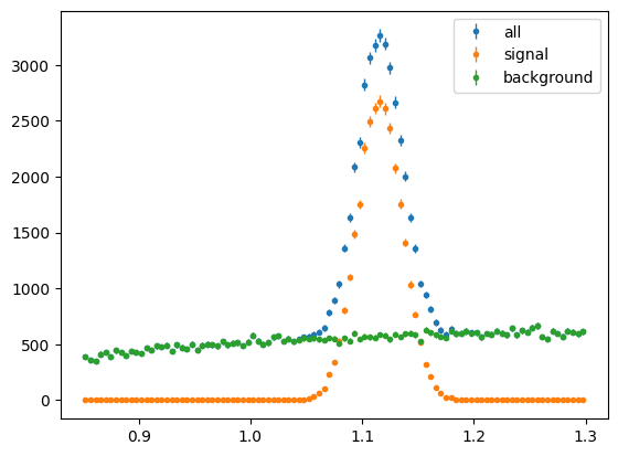
First we will import a simple toy data set for testing techniques on. This consists of 3 variables : mass, phi, and state. These will be loaded into 3 numpy arrays. The data consists of signal and background events with different mass and phi distributions for each.

mass: Gaussian signal, log background distributions
phi: Photon Asymmetry distribution \(1-h*\Sigma*\cos\left(2\phi\right)\) with different values of \(\Sigma\) for signal and background
state: magnitude =1 for signal, 2 for background. polarisation state, h = sign of state

/opt/hostedtoolcache/Python/3.10.14/x64/lib/python3.10/site-packages/gdown/cached_download.py:102: FutureWarning: md5 is deprecated in favor of hash. Please use hash='md5:xxx...' instead.
  warnings.warn(

data file :  [[ 1.18508   0.640313  1.      ]
 [ 1.01475   5.89936   2.      ]
 [ 0.983506  3.05945  -2.      ]
 ...
 [ 1.38359   6.13487  -2.      ]
 [ 1.36384   1.12189  -2.      ]
 [ 1.12189   2.59683  -2.      ]]
phi  [0.640313 5.89936  3.05945  ... 2.02081  4.4991   2.59683 ] 83156
mass  [1.18508  1.01475  0.983506 ... 1.24407  0.92379  1.12189 ] 83156
state  [ 1.  2. -2. ... -2.  2. -2.] 83156

Now we can plot each variable to see what we have. We will draw all, signal and background in different colours.

Note the histSqrtErrorBars is used to plot a histogram with error bars given by sqrt of the bin contents. This will not always be correct for the plots in this notebook.

First Mass:

_images/001fcae1aceeaf538cbbe14ed5c763f878d60ed61c0d977aaacd12d78dc0f661.png

Now phi

_images/eb82c4ae4b765ca99dfebcb3c912a33a44ce0076e38798b8c284782eac563b24.png

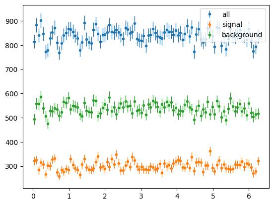
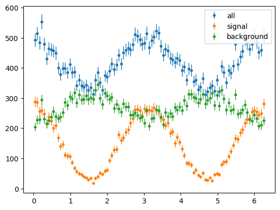
The phi distributions were flat as we summed over polarisation state h. Lets select only +ve h, i.e. +ve state

_images/85d900d2d4107775152fbb41cfc014b2fda49aeb21644f003676bfa4a36a0ec3.png

<Figure size 640x480 with 0 Axes>

Now we see we have cos2ϕ distributions with signal having a larger asymmetry and background having a different signed asymmetry.

Extended Maximum Likelihood Fit of Signal ϕ distribution#

Lets try some likelihood fits to see if we can estimate \(\Sigma\) for the signal. For simplicity we will assume only a single +ve polarisation state with degree of linear polarisation = 1.

(* Note normally we would see parallel or perpindicular polarisation states, but for ease of writing we use +ve and -ve labels instead.)

First we must define our PDF. This is just based on a photon asymmetry distribution as seen in earlier lectures.

\[ \frac{d\sigma(\phi:\Sigma)}{d\phi} = \sigma_{0}(1 - \Sigma \cos(2ϕ)) \]

As seen the normalisation integral for this functions is \(\sigma_{0}/2\pi\). Hence our PDF,

\[ p(\phi:\Sigma) = \frac{1}{2\pi}(1 - \Sigma \cos(2ϕ)) \]

Although more generally I could have the phi fit range instead of \(2\pi\).

def PhotonAsymmetryPDF(xphi, Sigma):
    """Photon Asymmetry PDF"""
    return (1 - Sigma * np.cos(2 * xphi)) / 2 / np.pi


def PhotonAsymmetryN(xphi, Sigma, N):
    """Unormalised Photon Asymmetry"""
    return N * PhotonAsymmetryPDF(xphi, Sigma)


def PhotonAsymmetryNExt(xphi, Sigma, N):
    """Unormalised Photon Asymmetry for extended maximum likelihood"""
    return (N, N * PhotonAsymmetryPDF(xphi, Sigma))

And lets plot this on the signal data

# Filter +ve polarisation signal events
sig_pos_mass = mass[state == 1]
sig_pos_phi = phi[state == 1]

bg_pos_mass = mass[state == 2]
bg_pos_phi = phi[state == 2]

print("Number of +νₑ signal events in our data = ", sig_pos_phi.size)

Number of +νₑ signal events in our data =  14938

Now to estimate the height of the function for the histogram, I know I have approximaely 15,000 events and 100 bins. So average height = 150. So I might guess I can just multiply my function by 150. But if I am using the PDF I must also scale by the \(2\pi\) factor.

\(\Sigma\) looks large and -ve so I will guess 0.7 for its value.

_images/adb35406822c844eeb79a6a1c231a0f929f6cb5f96e9956b2a95f571fab22116.png

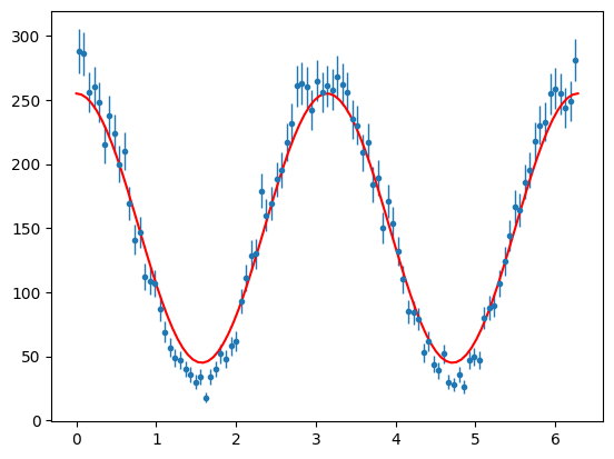
So the guess was reasonable. But lets find the best values using Maxmimum Likelihood.

I need to import minimisation classes. For these exercises we will use the iminuit package to perform a gradiant decent minimisation algorithm, migrad. Understanding this algorithm is very worthwhile, but not something we will cover here. Also there are other gradiant decent algothims available as well as completeley different methods such as genetic algorithms, or Bayesian methods such as MCMC or Nested Sampling which are also worth looking into for you own projects.

from iminuit import Minuit
from iminuit.cost import ExtendedUnbinnedNLL, UnbinnedNLL

Now I need to give Minuit a function to minimise. This function is the negative log likelihood for my PDF summing over the data

\[ \mathcal{L}(\theta_{j})=-\ln(L(\theta_{j})) = - \sum_{k}^N \ln[p(x_{i,k}:\theta_{j})] = - \sum_{k}^N \ln[\frac{1}{2\pi}(1 - \Sigma \cos(2ϕ))] \]

Ndata = sig_pos_phi.size

# mi = Minuit( ExtendedUnbinnedNLL(phi[state==1], PhotonAsymmetryN), sigma=-0.70, N = Ndata )
mi = Minuit(UnbinnedNLL(sig_pos_phi, PhotonAsymmetryPDF), Sigma=-0.70)

# set some physical limits on parameters
# mi.limits['N'] = (0,Ndata*1.1)
mi.limits["Sigma"] = (-1, 1)

And then I can perform the migrad algorithm. Here I will also use the hesse method for better uncertainty estimation.

Make sure you understand both algorithms, e.g. Hesse and Minos.

mi.migrad()
mi.hesse()

display(mi)

# save best estimate of Sigma to bestSigma
bestSigma = mi.values[0]
bestSigmaErr = mi.errors[0]
# Nminuit = mi.values[1]

print("Best value found for Sigma = ", bestSigma, "+-", bestSigmaErr)

Migrad
FCN = 4.977e+04	Nfcn = 19
EDM = 2.02e-05 (Goal: 0.0002)
Valid Minimum	Below EDM threshold (goal x 10)
No parameters at limit	Below call limit
Hesse ok	Covariance accurate

	Name	Value	Hesse Error	Minos Error-	Minos Error+	Limit-	Limit+	Fixed
0	Sigma	-0.792	0.008			-1	1

	Sigma
Sigma	6.63e-05

Best value found for Sigma =  -0.7924352797328573 +- 0.008143530773786933

I should have got a value close to (within 1 or 2 standard deviations) of \(\Sigma = -0.8\).

Note the displayed histrogram from iminuit does not attempt to give a very good comparison. You need to draw a new histogram with the result superimposed. As this was not an extended maximum likelihood fit, the normalisation was not determined. We must calculate this ourselves from the number of events (dividing by nbins and scaling by 2π).

_images/c14f8b420f22b2cd8f1da28eaad2b8a1aa73d81da2b525658879c56c9f335d5a.png

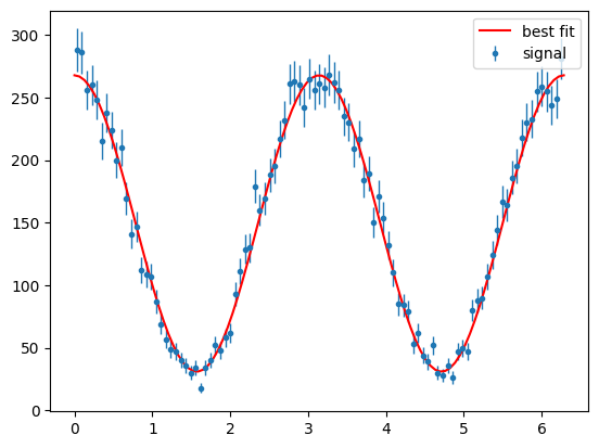
This looks good.

But the problem with data is I cannot normally seperate signal so easily. I need to use a discriminatory variable in some way. Next we will look at background subtractions via sPlots.

Signal and Background fit to Mass distribution#

In this example my discriminatory variable is going to be the mass distribution. This has distinct signal (Gaussian) and background (Unknown) components.

from scipy.stats import norm

Signal Distribution#

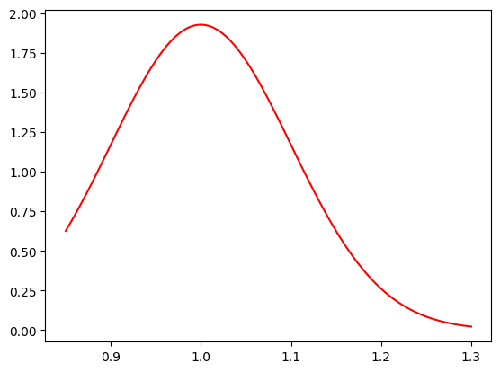
To define my signal PDF I can start from scipy norm distribution. However remember the PDF normalisation integral must be calculated within the fit ranges. Therefore I only need the integral of the distribution within these bounds rather than -∞ to ∞

To get this I just use the difference of the Cumulative Density Function at the fit limits, which for the normal distribution is analytically known.

_images/4e320e07d86482a0503da6930f7d843afadd0b135d1463aa3348aeb5b4505cba.png

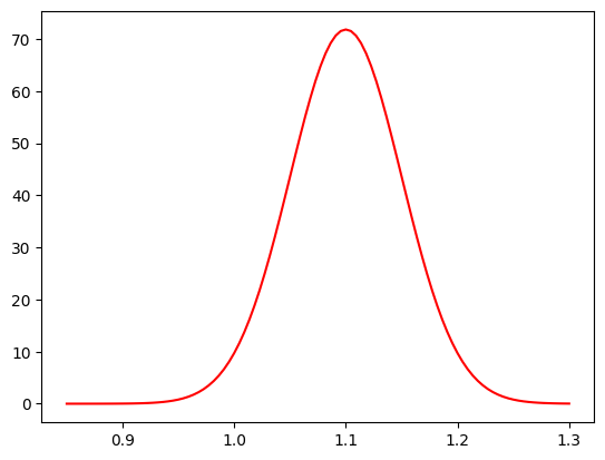
Here we are going to use Extended Maximum Likelihood for our fits as it is required for the sPlot covariance matrix.

So I need to define a function for iminuit.cost.ExtendedUnbinnedNLL, which just multiplies the PDF by the yield

_images/6a08c8e3561a8b2001ac9b96a87949b16f29879b6251926cb15002bd020081d7.png

And do the fit with iminuit:

Migrad
FCN = -3.079e+05	Nfcn = 84
EDM = 2.43e-06 (Goal: 0.0002)
Valid Minimum	Below EDM threshold (goal x 10)
No parameters at limit	Below call limit
Hesse ok	Covariance accurate

	Name	Value	Hesse Error	Minos Error-	Minos Error+	Limit-	Limit+	Fixed
0	mean	1.11560	0.00016			0.85	1.3
1	width	20.02e-3	0.12e-3			0.01	0.45
2	Ns	14.94e3	0.12e3			0	1.64E+04

	mean	width	Ns
mean	2.68e-08	0 (0.002)	-0
width	0 (0.002)	1.34e-08	-0
Ns	-0	-0	1.49e+04

Best value for mean =  1.115599505696138 +- 0.0001638406396170522
Best value for width =  0.020024762538705436 +- 0.0001158527420533316
Best value for yield =  14938.189483459864 +- 122.21049038349156

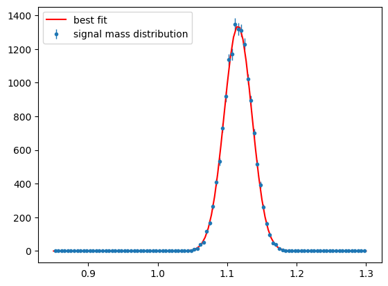
I should get a mean around 1.1, width around 0.02 and a signal yield of around my number of data events ~15,000.

The iminuit plot may not always looks like a great fit, it is not meant to give a correct comparison. Best to redraw the function with the best values to check the fit.

Note this time the normalisation has been determined by the extended fit and I just need to account for the number of bins in my histogram.

_images/1f6a25597e81c3627ba0a95f5c0bec23b5c92f87c8f7924d8f086f228ba59399.png

Background Distribution#

Often background distributions will not have a well defined PDF shape. As a proxy polynomial distributions can be used instead. This is likely to induce some systematic uncertainty in the final results due to mismodelling of the discriminatory variable fit, which should be investigated/estimated.

When fitting polynomials as PDFs it is often the Chebyshev form of the polynomials which is used. Here we will just use predefined functions for this.

Investigate or discuss why Chebyshev’s are better to use.

_images/f1d77a557355556072e09a5985e6ba561da040f1d35e1366fee44aac00a2b4c8.png

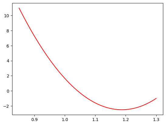
Watch out for -ve PDF values, these are not allowed and will screw up the minimisation. In practise we should edit our function to protect against this. Here it turn out not to be an issue, (we fix c0=1) but in general IT WILL BE!

Now define my function for ExtendedUnbinnedNLL

def BgMassNExt(xmass, c0, c1, c2, c3, c4, Nb):
    # limit it to max 5 polynomial terms
    return (Nb, Nb * ChebPDF(xmass, [c0, c1, c2, c3, c4]))

Migrad
FCN = -4.882e+05	Nfcn = 108
EDM = 2.15e-05 (Goal: 0.0002)
Valid Minimum	Below EDM threshold (goal x 10)
No parameters at limit	Below call limit
Hesse ok	Covariance accurate

	Name	Value	Hesse Error	Minos Error-	Minos Error+	Limit-	Limit+	Fixed
0	c0	1.00	0.01			-1	1	yes
1	c1	0.203	0.012			-1	1
2	c2	-0.063	0.011			-1	1
3	c3	0.016	0.010			-1	1
4	c4	0.0	0.1			-1	1	yes
5	Nb	26.55e3	0.16e3			0	2.92E+04

	c0	c1	c2	c3	c4	Nb
c0	0	0	0	0	0	0
c1	0	0.000145	0.01e-3 (0.101)	0.06e-3 (0.483)	0	-0
c2	0	0.01e-3 (0.101)	0.000114	0.01e-3 (0.106)	0	-0
c3	0	0.06e-3 (0.483)	0.01e-3 (0.106)	0.000105	0	-0
c4	0	0	0	0	0	0
Nb	0	-0	-0	-0	0	2.66e+04

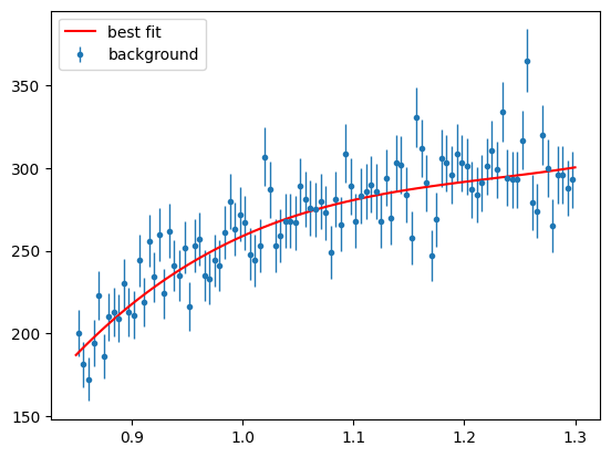
And draw the fit result with the data

_images/a2fa9b80ba78874984d2ef4a6b5609a896a4d8203bcdca1bbdf3af65188b6ff5.png

Simulated Signal and Background PDFs#

Aside : It is not always the case that a signal peak will be well fitted by a Gaussian distribution, or that a background can be easily constrained to a polynomial. In general simulations may give the best approximate PDF shapes for your event types.

Practically how may you generate a PDF using simulated data? What do you need and what might be the problems?

Joint fit to 1D Signal and Background#

We now have our signal and background PDF functions (\(p_s\) and \(p_b\)) which we can use in Extended Maximim Likelihood fits. To proceed we must first combine this into a single distribution for fitting i.e.

\[ f(m:Y_s,Y_b,\mu_s,\sigma_s,c1_b,c2_b,c3_b,c4_b) = Y_s p_s(m:\mu_s,\sigma_s) + Y_b p_b(m:c1_b,c2_b,c3_b,c4_b) \]

Where \(Y_{s,b}\) are the expected signal and background yields in the data. We then need to perform a full fit for all parameters \(\theta_j = \{Y_s,Y_b,\mu_s,\sigma_s,c1_b,c2_b,c3_b,c4_b\}\)

def CombinedMassNExt(xmass, smean, swidth, bc0, bc1, bc2, bc3, bc4, Ys, Yb):
    return (
        (Ys + Yb),
        Ys * SignalMassPDF(xmass, smean, swidth)
        + Yb * ChebPDF(xmass, [bc0, bc1, bc2, bc4, bc4]),
    )

First make our combined data sets

# Filter all +ve polarisation events
pos_mass = mass[state > 0]
pos_phi = phi[state > 0]

print("Number of +ve  events in our data = ", pos_phi.size)

Number of +ve  events in our data =  41491

Now run iminuit with ExtendedUnbinnedNLL on our combined PDF and dataset

Migrad
FCN = -8.205e+05	Nfcn = 166
EDM = 2.61e-07 (Goal: 0.0002)	time = 0.3 sec
Valid Minimum	Below EDM threshold (goal x 10)
No parameters at limit	Below call limit
Hesse ok	Covariance accurate

	Name	Value	Hesse Error	Minos Error-	Minos Error+	Limit-	Limit+	Fixed
0	smean	1.11569	0.00023			0.85	1.3
1	swidth	19.93e-3	0.21e-3			0.01	0.45
2	bc0	1.00	0.01			-1	1	yes
3	bc1	0.204	0.011			-1	1
4	bc2	-0.062	0.012			-1	1
5	bc3	-0.1	1.5			-1	1
6	bc4	15.71e-3	0.16e-3			-1	1	yes
7	Ys	14.81e3	0.17e3			0	9.15E+04
8	Yb	26.69e3	0.20e3			0	9.15E+04

	smean	swidth	bc0	bc1	bc2	bc3	bc4	Ys	Yb
smean	5.11e-08	0 (0.001)	0	-0.13e-6 (-0.051)	-0.16e-6 (-0.056)	0	0	-459.26e-6 (-0.012)	114.49e-6 (0.003)
swidth	0 (0.001)	4.63e-08	0	-0.23e-6 (-0.097)	0.77e-6 (0.285)	0	0	14.66084e-3 (0.399)	-14.59971e-3 (-0.338)
bc0	0	0	0	0	0	0	0	0	0
bc1	-0.13e-6 (-0.051)	-0.23e-6 (-0.097)	0	0.000125	-0.01e-3 (-0.046)	0	0	-293.82e-3 (-0.154)	185.53e-3 (0.083)
bc2	-0.16e-6 (-0.056)	0.77e-6 (0.285)	0	-0.01e-3 (-0.046)	0.000156	0	0	755.95e-3 (0.355)	-739.65e-3 (-0.295)
bc3	0	0	0	0	0	1.99	0	0.0	0.0
bc4	0	0	0	0	0	0	0	0	0
Ys	-459.26e-6 (-0.012)	14.66084e-3 (0.399)	0	-293.82e-3 (-0.154)	755.95e-3 (0.355)	0.0	0	2.91e+04	-0.013e6 (-0.388)
Yb	114.49e-6 (0.003)	-14.59971e-3 (-0.338)	0	185.53e-3 (0.083)	-739.65e-3 (-0.295)	0.0	0	-0.013e6 (-0.388)	4.02e+04

And plot the fit result

_images/43f95a130b96ad204038002d84439f328e05509022f281d6d7bf76f16605ab22.png

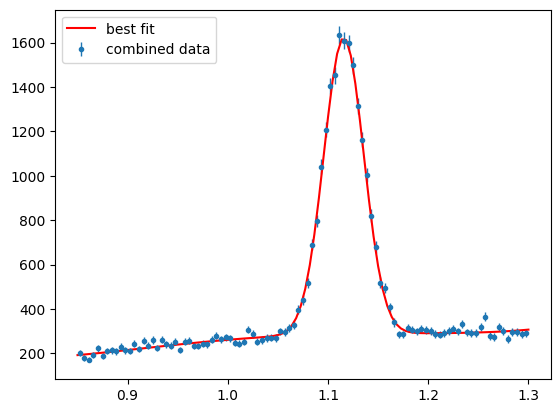
The fit should be pertty good although the polynomial background does not get such a good job close to threshold, if that is included in the range (Should be at 0.8). If the fit was succesfull then the results can now be used to generate weights for background subtraction (e.g. Sidebands or sPlots).

sPlots#

We are going to use the sweights library provided by https://sweights.readthedocs.io/en/latest/about.html This is related to the referenced paper on Custom Orthogonal Weight functions, of which sPlots is a specific case of. https://www.sciencedirect.com/science/article/pii/S0168900222006076?via%3Dihub

One issue with sweights is it requires zero dependence between the discriminatory and physics variables used and this is often not the case. The COWS method suggests a solution for the case where there is a dependence, but it is beyond the scope of these lectures.

In our toy dataset the discrimiatory (mass) and physics(phi) variables are independent for both signal and background events.

from sweights import SWeight  # for classic sweights

Remember the sWeights formula,

\[ w_{t,k} = \frac{\sum_{t'}^{N_{t}} V_{tt'}.P_{t'}(x_{k}) }{\sum_{t'}^{N_{t}} Y_{t'}.P_{t'}(x_{k})} \]

The SWeight() function will calculate the covariance matrix,

\[ \left[ V_{tt'} \right]^{-1} = \frac{\partial ^2 \mathcal{ L}(\theta^{best}_{j},Y_{t})}{\partial Y_{t}Y_{t'}} = \sum^{N_{k}}_{k}\frac{P_{t}(x_{k})P_{t'}(x_{k})}{\left( \sum_{t'}^{N_{t}} Y_{t'}.P_{t'}(x_{k}) \right)^{2}} \]

It can use either method, taking the approximate partial derivitives from a extended maximum likelihood fit, with method=”roofit” \(^{note}\) (left option) or by summing over the data events k with method=”summation” (right option).

This is indeed what RooFit does and the implementation just calls RooFit, however you need RooFit imported for that, which is not possible within Colab currently.

# create best value PDFs for signal and background
spdf = lambda m: SignalMassPDF(m, sg_mean, sg_width)
bpdf = lambda m: ChebPDF(m, [bg_c2, bg_c3, bg_c4, bg_c5])

# make the sweighter
# note here I am using the fits to the positive data
sweighter = SWeight(
    pos_mass,
    [spdf, bpdf],
    [Ysignal, Yback],
    (mrange,),
    method="summation",
    compnames=("sig", "bkg"),
    verbose=True,
    checks=True,
)

Initialising sweight with the summation method:
    PDF normalisations:
	 0 0.4499999999999992
	 1 0.4498687600447206
    W-matrix:
	[[4.91384538e-05 1.02267413e-05]
	 [1.02267413e-05 3.17906752e-05]]
    A-matrix:
	[[21810.91026572 -7016.35105054]
	 [-7016.35105054 33712.85448948]]

    Integral of w*pdf matrix (should be close to the
                identity):
	[[ 9.99941794e-01 -3.81009290e-04]
	 [-3.70663726e-04  1.00062027e+00]]
    Check of weight sums (should match yields):
	Component  | sWeightSum |   Yield    |   Diff    |
	---------------------------------------------------
	  0        | 14805.5884 | 14805.5884 |    -0.00% |
	  1        | 26685.4393 | 26685.4393 |     0.00% |

Plot the weights

_images/9f7609a247ed243f505346ed9cd5e7bc7144bbbf2776a317a3ad12a91362e802.png

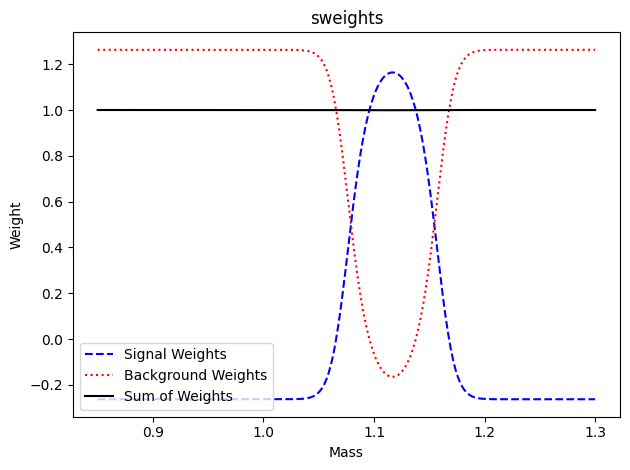
Discuss if these weights look reasonable. Why are Signal Weights <0 in some regions?

Now plot the weighted phi distributions for the +ve polarisation data

_images/cae3512e32f963a094e3738cf8aa9f1a93d8bda84692606470dc5cf418dec3dd.png

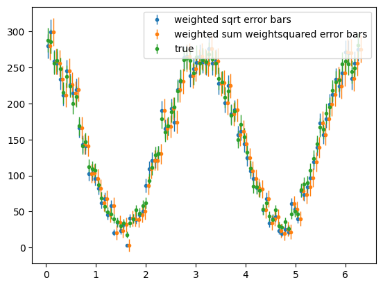
Investigate or discuss if these distributions and error bars look OK. Which are the correct error bars for the weighted data, blue or orange? Should weighted data have same, smaller or larger error bars than true signal events?

Exercise 14

Make phi plots for background distributions

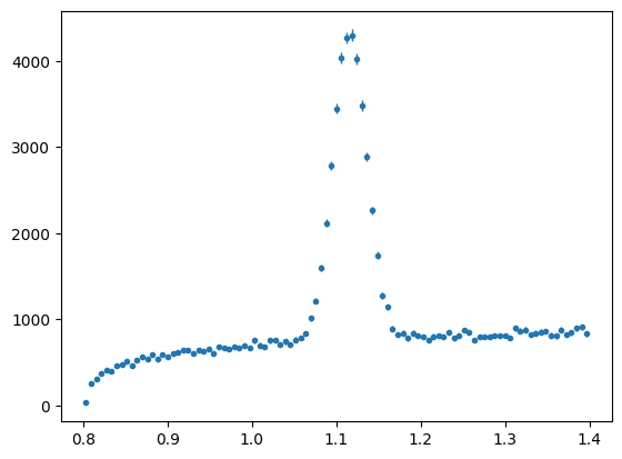
Lets consider the full mass range in the data file (draw with the next cell). We have restricted it in our test data and fits so far. Why might we a) restrict the range? b) use as large a range as we can?.

fullrange = np.linspace(0.8, 1.4, 100)
mass_hist = s2020.histSqrtErrorBars(dataArray[:, 0], fullrange, "fullrange")

_images/8e64377146780eec4d6399f15d6168f0f86e7f9a2c36c212bb1bba14feca3bb4.png

Inclusion of Weights in Maximum Likelihood#

We will again fit the Photon Asymmetry to extract \(\Sigma\), but now we will disentangle the signal response using the sWeights in the fit.

Here we need to define our own loss function where the log likelihood values are weighted with our background subtraction weights.

The weighted negative log likelihood function,

\[ \mathcal{L}(\theta_{j}) = - \sum_{k}^{N_{k}} w_{k} \ln[ p(x_{Pi,k}:\theta_{Pj})] = - \sum_{k}^{N_{k}} w_{k} \ln[ p(\phi_{k}:\Sigma)] \]

# NLL for maximum likelihood with weights
# Sigma = parameter to fit
# data_phi = array of phi data
# wk weights for signal (or background)


def PhotonAsymWeightedNLL(Sigma, data_phi, wk):
    pdf_vals = PhotonAsymmetryPDF(data_phi, Sigma)
    return -np.sum(wk * np.log(pdf_vals))

And perform the fit with iminuit:

Migrad
FCN = 2.454e+04	Nfcn = 24
EDM = 1.77e-06 (Goal: 0.0001)
Valid Minimum	Below EDM threshold (goal x 10)
No parameters at limit	Below call limit
Hesse ok	Covariance accurate

	Name	Value	Hesse Error	Minos Error-	Minos Error+	Limit-	Limit+	Fixed
0	Sigma	-0.813	0.008			-1	1

	Sigma
Sigma	6.45e-05

best value for background subtracted Sigma =  -0.8128619781253672 +- 0.008030047587728684

How do the results and uncertainties compare to the signal only fitting? Does this seem reasonable?

print("best value for signal only data Sigma = ", bestSigma, "+-", bestSigmaErr)

best value for signal only data Sigma =  -0.7924352797328573 +- 0.008143530773786933

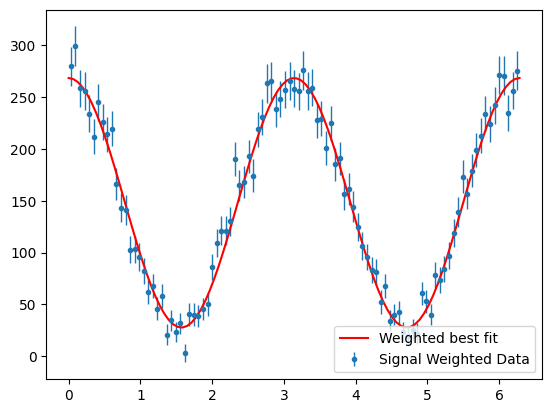
Now we can plot the fit result with the background subtracted data.

signal yield :  14805.588384960924

_images/2a37253e57c0b43dc6862af6309557e70722756a0f17ab0450f225628a268abb.png

Uncertainties in Weighted Maximum Likelihood fits#

In general correctly accounting for the effect of the weights on the uncertainties is a non-trivial task. For in-depth discussion of the asymptotically correct method see “Parameter uncertainties in weighted unbinned maximum likelihood fits”, Langenbruch, https://epjc.epj.org/articles/epjc/abs/2022/05/10052_2022_Article_10254/10052_2022_Article_10254.html

We will test the simplest method given therein, which is not in general correct, but can give a good approximation. It has been used in many publications. That is to add an additional factor to the sum of logs in the likelihood,

\[ \mathcal{L}(\theta_{j}) = - \frac{\sum_{k}^{N_{k}} w_{k}}{\sum_{k}^{N_{k}} w_{k}^{2}} \sum_{k}^{N_{k}} w_{k} \ln[ p(x_{Pi,k}:\theta_{Pj})] \]

You should see a similarity between this “sum of weights, over, sum of weights squared” factor and our histogram uncertainties.

# NLL for maximum likelihood with weights
# See Langenbruch (19)


def PhotonAsymWeightedW2WNLL(Sigma, data_phi, wk):
    pdf_vals = PhotonAsymmetryPDF(data_phi, Sigma)
    yld = np.sum(wk)
    sw2 = np.sum(wk * wk)
    # sum of weights/ sum of weights squared correction factor
    return -(yld / sw2) * np.sum(wk * np.log(pdf_vals))
    # + N - yld*np.log(N))

nllw2w = lambda Sigma: PhotonAsymWeightedW2WNLL(Sigma, pos_phi, sig_weights)
mi = Minuit(nllw2w, Sigma=0.1)
mi.errordef = Minuit.LIKELIHOOD

mi.limits["Sigma"] = (-1, 1)
mi.migrad()
mi.hesse()
display(mi)

print(
    "best value for background subtracted Sigma with sumw2 correction = ",
    mi.values[0],
    "+-",
    mi.errors[0],
)

Migrad
FCN = 1.666e+04	Nfcn = 24
EDM = 1.2e-06 (Goal: 0.0001)
Valid Minimum	Below EDM threshold (goal x 10)
No parameters at limit	Below call limit
Hesse ok	Covariance accurate

	Name	Value	Hesse Error	Minos Error-	Minos Error+	Limit-	Limit+	Fixed
0	Sigma	-0.813	0.010			-1	1

	Sigma
Sigma	9.5e-05

best value for background subtracted Sigma with sumw2 correction =  -0.8128619781294631 +- 0.00974620788177144

As mentioned this may be a reasonable approximation (or not) but it does not fully propogate the uncertainty. For example the uncertainty on our signal PDF parameters (mean and width) are not incorporated. Next we consider bootstrapping, which is a more time-consuming, but more robust method, for determining uncertainties as sample distributions. Note that incoporporating the sigal PDF parameter uncertainties will be left as an exercise (2).

More Uncertainties : Bootstrapping#

As outlined in the Langenbruch paper, Bootstrapping provides another independent method for estimating the uncertainties.

In the paper two variations are performed

Boot strap the data and use the same weights
Bootstrap the data and redo the sPlot fits.

Here we will follow (1) with (2), the better method, left as an exercise.

Bootstrapping involves refitting the data many times. Each time using a different selection of events. Events are sampled from the original data set and crucially (to get correct variance) the sampling is done with replacements (i.e. 1 event is chosen from the same Nk events for each event in the bootstrapped data set). The point estimates of the fit results can then be used to construct the standard deviation or confidence levels. Pretty simple, bruteforce, effective!

To achieve an accurate estimate of the uncertainty a large number \(O(10,000)\) of bootstrap samples should be fit.

You can search the web to find more about bootstrapping for uncertainties, it is a common tool.

Algorithm :

Sample \(N_{k}\) events (or a fraction of) from the \(N_{k}\) data events \(N_{boot}\) times.
Each time refit the sampled data and save the result.

We have a couple of control parameters,

Nboot The number of bootstrap fits to perform
frac_to_sample: The fraction of \(N_{k}\) events to use in each new bootstrap data sample

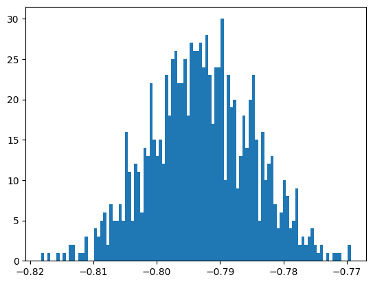
Bootstrap Signal Only Data#

First we can validate the mothod using fits to signal only data, and check we get a consistent uncertainty as we did in “Extended Maximum Likelihood Fit of Signal ϕ distribution”

# data_phi_sig_para = phi[state==1]
Nk = sig_pos_phi.size

Nboot = 1_000
frac_to_sample = 1.0 / 1

# calc, number of events per bootstrap sample
# this could be = Nk
Nsamp = int(Nk * frac_to_sample)

# create list to save bootstrap results
bt_sigmas = []

# loop over Nboot samples
for bt in range(Nboot):
    # use random choice to do sampling with replacements
    phi_bt = np.random.choice(sig_pos_phi, Nsamp)

    # and do the fit for this bootstrap sample
    btmi = Minuit(UnbinnedNLL(phi_bt, PhotonAsymmetryPDF), Sigma=-0.5)
    btmi.limits["Sigma"] = (-1, 1)
    btmi.migrad()
    # save results, only care about best fit value
    bt_sigmas.append(btmi.values[0])
bt_sigmas = np.array(bt_sigmas)

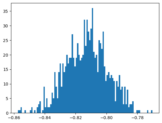
plt.hist(bt_sigmas, bins=100)
print("the mean of bootstrap samples = ", bt_sigmas.mean())
print("the standard deviation of bootstrap samples = ", bt_sigmas.std())
print(
    "the scaled standard deviation of bootstrap samples = ",
    bt_sigmas.std() * np.sqrt(frac_to_sample),
)

the mean of bootstrap samples =  -0.7929227048250925
the standard deviation of bootstrap samples =  0.008002333357563726
the scaled standard deviation of bootstrap samples =  0.008002333357563726

_images/4072592451b57d2dd56c17a2eed0d07889a85d4149e3fb43c7ca1b281528377c.png

Why multiply the standard deviation by sqrt(frac_to_sample)?

Exercise 15 (Complete the tables)

Best/mean value of \(\Sigma\) from iminuit and bootstrapping.

Nboot / frac	1/4	1/16
`iminuit`	-	-
10
100
1,000
5,000

Uncertainties on \(\Sigma\) from iminuit and bootstrapping.

Nboot / frac	1/4	1/16
`iminuit`	-	-
10
100
1,000
5,000

Bootstrap Background Subtracted Data#

Now we want to try bootstrapping on the background subtracted fits to test our uncertaintiy estimates.

Algorithm :

Sample \(N_{k}\) events (or a fraction of) from the \(N_{k}\) data events \(N_{boot}\) times.
Each time calculate the sPlot weights for the sampled data
Then refit the sampled data using weighted nll and save the result.

This is slower, so do not try too many boots.

# remember to get signal weights we use sig_weights  = sweighter.get_weight(0, para_mass)
# i.e. we are using the sweighter configured from the fit already done in "sPlots"

# remember data is pos_phi and pos_mass

Nk = pos_phi.size

Nboot = 1_000
frac_to_sample = 1.0 / 1
Nsamp = int(Nk * frac_to_sample)

bt_wgted_sigmas = []

# now we need to synchronise our bootstrap samples of mass and phi
# so we instead choose to sample the array indices
all_indices = np.arange(Nk)

for bt in range(Nboot):
    indices_bt = np.random.choice(all_indices, Nsamp)
    wgts_bt = sweighter.get_weight(0, pos_mass[indices_bt])
    # now need to create nll
    btnll = lambda Sigma: PhotonAsymWeightedNLL(Sigma, pos_phi[indices_bt], wgts_bt)
    btmi = Minuit(btnll, Sigma=-0.1)
    btmi.limits["Sigma"] = (-1, 1)
    btmi.migrad()
    bt_wgted_sigmas.append(btmi.values[0])
bt_wgted_sigmas = np.array(bt_wgted_sigmas)

plt.hist(bt_wgted_sigmas, bins=100)
print("the mean of bootstrap samples = ", bt_wgted_sigmas.mean())
print("the standard deviation of bootstrap samples = ", bt_wgted_sigmas.std())
print(
    "the scaled standard deviation of bootstrap samples = ",
    bt_wgted_sigmas.std() * np.sqrt(frac_to_sample),
)

the mean of bootstrap samples =  -0.8128769400190295
the standard deviation of bootstrap samples =  0.013606270180531354
the scaled standard deviation of bootstrap samples =  0.013606270180531354

_images/820f9404778dfb7ebfff280da36db5abdf6411d43eb99b50f0530359423abba3.png

Exercise 16

Complete the tables, using result from “Uncertainties in Weighted Maximum Likelihood fits

Best/mean value of \(\Sigma\) from weighted fits using iminuit and bootstrapping.

Nboot / frac	1/4	1/16
`iminuit`	-	-
10
100
1,000

Uncertainties on \(\Sigma\) from weighted fits using iminuit and bootstrapping. Give corrected (sum of weights over sum of weights squared) and uncorrected uncertainties for iminuit

Nboot / frac	1/4	1/16
`iminuit` uncor	-	-
`iminuit` cor	-	-
10
100
1,000

Correcting for Acceptance#

Acceptance refers to the probabilty of detecting and reconstructing your reaction at a given point in variable space \(x_{i,k}={x_{0,k},x_{1,k},x_{2,k}...}\). The \(x_{i,k}\) may be any measured (e.g momentum) or calculated variable (e.g. invariant mass). It can be given by the ratio of all events to those detected and reconstructed (aka accepted).

\[ η(x_{i,k}) = \frac{f_{acc}(x_{i,k})}{f_{all}(x_{i,k})} \approx \frac{N^{MC}_{acc}(x_{i,l})}{N^{MC}_{gen}(x_{i,l})} \]

This acceptance is generally approximated through Monte-Carlo simulations of detector setups. To actually calculate a value for \(η(x_{i,k})\) requires some integration of MC events \(x_{i,l}\) sufficiently local to \(x_{i,k}\). This can be problematic if \(N_{i} > 2\), i.e. if we need an acceptance in high dimensions.

Maximum Likelihood to the rescue!#

In turns out, somewhat magically, the maximum likelihood method removes the need to determine \(η(x_{i,k})\) for each event. It essentially just requires a single integration over full \(x_{i,k}\) space. Now, in general, the integration needs to be done for every value of model parameters (used in the fitting) instead. This however can be done more accurately, than individual acceptances, for a given number of MC events.

Lets look at the equations. I have some function which describes my data that now depends on some physics model \(I(x_{i}:\theta_{j})\) and some detector acceptance \(\eta(x_{i})\),

\[ f(x_{i}:\theta_{j}) = I(x_{i}:\theta_{j}).\eta(x_{i}) \]

Then I can calculate my PDF using a numerical calculation of the normalisation integral which is a summation over all \(M\) accepted MC simulation events.

\[ p(x_{i}:\theta_{j}) = \frac{I(x_{i}:\theta_{j})\eta(x_{i})}{ \sum^M_l I(x_{i,l}:\theta_{j}) } \]

Note, η is not required in the summation as it is explicitly included in the accepted events \(M\), which is less than the number of generated MC (or thrown) events.

\[\begin{split} \begin{eqnarray} L(\theta_{j},Y) &=& \prod_{k=0}^N p(x_{i,k}:\theta_{j}) \\ -\ln L(\theta_{j},Y) &=& - \sum_{k=0}^N \ln[\frac{I(x_{i,k}:\theta_{j})}{ \sum^M_l I(x_{i,l}:\theta_{j})}] - \sum_k^N \ln{\eta(x_{i,k})} \end{eqnarray} \end{split}\]

Now we observe the last term (summing logs of acceptance) does not depend on our model parameters \(\theta_j\). Hence it is constant and can be ignored in the minimisation. The sum over \(l\) MC events does depend on the parameters and so this must be recalculated for each parameter set in the minimisation.

Toy Acceptance Model#

The data we have used so far has been “perfectly” detected. to investigate acceptance effects we need to add in these to the data. To do this we will just define some simple ϕ dependent functions, with some degraded acceptance or holes.

def AcceptanceFilter(darr, condarr, acc_func):
    """Function to filter the data to mock up the acceptance

    darr = data array to be filtered
    condarr = data array with which to test the acceptance (does not have to be same as darr)
    acc_func = takes a data array and returns a probability of being accepted for each entry
    """
    rands = np.random.uniform(0, 1, condarr.size)
    mask = rands[:] < acc_func(condarr)
    return darr[mask]


def PhiAcceptHoleFunc(phi_vals):
    """An acceptance function with just a hole."""
    return (phi_vals > 1) & (phi_vals < 2)


def PhiAcceptSinFunc(phi_vals):
    """An acceptance function with a sin phi dependence"""
    return np.sin(0.5 * phi_vals)

_images/3eb97a0a67bbdd820b3f4a7b0145dc08eb9653058488a46d4dcb6228e3156894.png

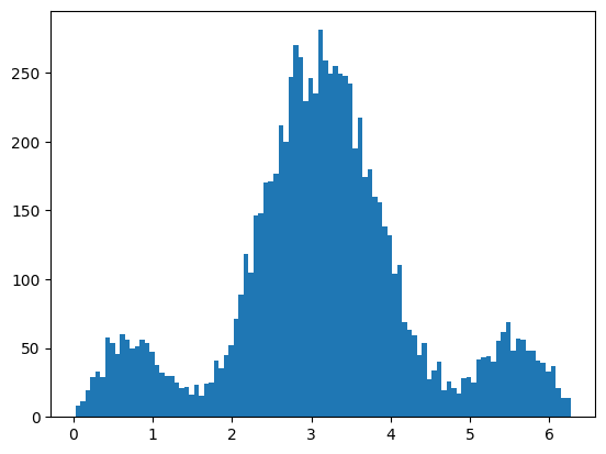
ndata 8946

Now lets try fitting the filtered data ignoring the acceptance.

Migrad
FCN = 3.055e+04	Nfcn = 28
EDM = 1.17e-06 (Goal: 0.0002)
Valid Minimum	Below EDM threshold (goal x 10)
No parameters at limit	Below call limit
Hesse ok	Covariance accurate

	Name	Value	Hesse Error	Minos Error-	Minos Error+	Limit-	Limit+	Fixed
0	Sigma	-0.719	0.012

	Sigma
Sigma	0.000143

Best value found for Sigma =  -0.7185348281657622 +- 0.011939017027492461

This should probably be significantly removed from the true value of -0.8. Also the plots do not match at all (allthough we should not take them too seriuosly)

Now lets try applying weights to correct for acceptance. This is different from the method discussed about, but since we can analyitically calculate the weights we might as well see how it does.

i.e. we are going to use a likelihood like,

\[ -\ln L(\theta_{j},Y) = - \sum_{k=0}^N \ln[\frac{p(x_{i,k}:\theta_{j})\eta(x_{i,k})}{\eta(x_{i,k})}] \]

Migrad
FCN = 1.242e+04	Nfcn = 24
EDM = 8.41e-08 (Goal: 0.0002)
Valid Minimum	Below EDM threshold (goal x 10)
No parameters at limit	Below call limit
Hesse ok	Covariance accurate

	Name	Value	Hesse Error	Minos Error-	Minos Error+	Limit-	Limit+	Fixed
0	Sigma	-0.792	0.016			-1	1

	Sigma
Sigma	0.000268

Best value found for Sigma =  -0.7916920884052856 +- 0.016368716352203216

This should give a value much closer to -0.8.

Now we can try our normalisation integral method.

For this we will define a new PDF for the Photon Asymmetry where we include the acceptance in the normalisation integral.

Here I am just calculating the function value at regular intervals along its range. To be more in line with using MC data I could have generated random points and used those instead.

Exercise 17

Try switching to random samples rather than regular arrays for the numeric integration.

# include acceptance in normalisation integral
integral_edges = np.arange(0, 2 * np.pi, 0.001)
integral_centres = (integral_edges[:-1] + integral_edges[1:]) / 2


def PhotonAsymAccPDF(xphi, Sigma):
    # evaluate PDF over samples
    vals = PhotonAsymmetryPDF(integral_centres, Sigma)
    # evaluate acceptance function over samples
    accs = PhiAcceptSinFunc(integral_centres)
    # sum to get integral
    integ = np.sum(vals * accs) / integral_centres.size
    # return value of PDF
    return PhotonAsymmetryPDF(xphi, Sigma) / integ

Now use this PDF with acceptance in normalisation integral in the likelihood fit.

Migrad
FCN = -1.134e+04	Nfcn = 31
EDM = 5.57e-08 (Goal: 0.0002)
Valid Minimum	Below EDM threshold (goal x 10)
No parameters at limit	Below call limit
Hesse ok	Covariance accurate

	Name	Value	Hesse Error	Minos Error-	Minos Error+	Limit-	Limit+	Fixed
0	Sigma	-0.793	0.010

	Sigma
Sigma	9.83e-05

Best value found for Sigma =  -0.7934383115571435 +- 0.009916664391627666

Hopefully the value has turned out to be close to -0.8 again! But the uncertainty is different from the previous example where we divided out the acceptance.

Of course we have learnt that we may use Bootstrapping to check the uncertainties from likelihood minimisations. Lets try that here.

To make it neater lets define a bootstrapper function which takes the data with acceptance and a -ve log likelihood function.

def bootstrapper(all_data, Nboot, frac, nll):
    Nsamp = int(all_data.size * frac)

    bt_sigmas = []

    # bootstrap loop : sample, fit, store
    for bt in range(Nboot):
        phi_bt = np.random.choice(all_data, Nsamp)
        btmi = Minuit(nll(phi_bt), Sigma=0)
        btmi.migrad()
        bt_sigmas.append(btmi.values[0])
    bt_sigmas = np.array(bt_sigmas)

    # output results
    plt.hist(bt_sigmas, bins=100)
    print("\n the mean of bootstrap samples = ", bt_sigmas.mean())
    print("the standard deviation of bootstrap samples = ", bt_sigmas.std())
    print(
        "the scaled standard deviation of bootstrap samples = ",
        bt_sigmas.std() * np.sqrt(frac),
    )
    return np.array(bt_sigmas)

Checking normalisation integral method
Remember best value found for Sigma =  -0.7934383115571435 +- 0.009916664391627666

 the mean of bootstrap samples =  -0.7937714370153646
the standard deviation of bootstrap samples =  0.019519189478003993
the scaled standard deviation of bootstrap samples =  0.009759594739001997

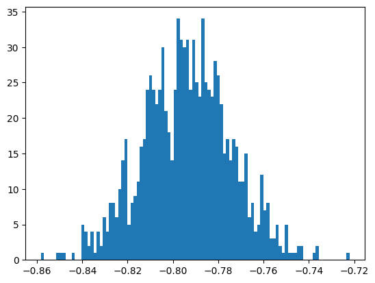
_images/d9e5132bc98106dd017feb71745991593e8bc368bc1c16f4f891c8d07a32c815.png

How does the bootstrap uncertainty compare to the iminuit one?

Further Exercises#

Exercise 18

Create weights for the data using a sideband method (see overview slides) and plot the sideband subtracted phi distributions. i.e. Redo the sPlots Section for sideband subtraction.
The data contain para and perp polarized data. Currently we have used just para.Write an expanded Photon Asymmetry function to include both polarisation states and fit the signal only data.
Now try applying the acceptance function to filter the data. Try fitting without applying any acceptance correction, what do you think you will get as a result?
For bootstrapping we do not reproduce the sWeights each fit. Should we? Include an sweight fit to the mass distributions of the bootstrap samples before the likelihood fit for the photon asymmetry. Algorithm:

Sample \(N_{k}\) events (or a fraction of) from the \(N_{k}\) data events \(N_\mathrm{boot}\) times.
Each time redo the sPlot Extended Maximum Likelihood fit and create new sweighter
Then calculate the sPlot weights for the sampled data
Finally, refit the sampled data using weighted nll, new weights and save the result.

Rather than subtracting background we may perform a simultaneous fit to both signal and background distributions dependent on the discriminatory variable and control variable, i.e. mass and phi. Deduce the combined PDF function and try fitting the data with it. How do the results compare, which should be more reliable? What is the advantage of seperating the discriminatory variable fit?