Lecture 12 – Computing angles#
Plot of angles in some reference systems: center-of-mass vs Gottfried-Jackson vs Adair
import gdown
import matplotlib.pyplot as plt
import numpy as np
import pandas as pd
from pylorentz import Momentum4
Again we download the data file using the gdown package:
output_path = gdown.cached_download(
    url="https://drive.google.com/uc?id=1qiYjPbR5nx3_Sw7MXuUKhNAUpkXPoxYh",
    path="data/gammapi_2pions_inclusive.dat",
    md5="38cf5bf915318df756a21a82ad9e4afa",
    quiet=True,
)
data = pd.read_csv(output_path)
data.columns = data.columns.str.strip()
data
/opt/hostedtoolcache/Python/3.10.14/x64/lib/python3.10/site-packages/gdown/cached_download.py:102: FutureWarning: md5 is deprecated in favor of hash. Please use hash='md5:xxx...' instead.
  warnings.warn(
| p1x | p1y | p1z | E1 | p2x | p2y | p2z | E2 | p3x | p3y | p3z | E3 | pgamma | helGamma | ||
|---|---|---|---|---|---|---|---|---|---|---|---|---|---|---|---|
| 0 | 0.517085 | 0.161989 | 0.731173 | 0.920732 | -0.254367 | 0.082889 | 0.495509 | 0.580189 | -0.259266 | -0.265152 | 0.445175 | 1.10275 | 1.657800 | -1 | |
| 1 | -0.216852 | -0.245333 | 0.107538 | 0.371878 | -0.183380 | 0.191897 | 0.145128 | 0.333213 | 0.389750 | 0.112110 | 0.790133 | 1.29195 | 1.044790 | -1 | |
| 2 | 0.197931 | 0.071432 | -0.010077 | 0.252778 | -0.111780 | -0.360482 | 0.367842 | 0.545221 | -0.090228 | 0.302313 | 0.724911 | 1.22694 | 1.095470 | -1 | |
| 3 | -0.505371 | -0.163949 | 0.450407 | 0.710395 | -0.141057 | 0.282404 | 1.186530 | 1.235730 | 0.679497 | -0.112014 | 0.729706 | 1.37371 | 2.388690 | -1 | |
| 4 | 0.260706 | -0.330303 | 0.385968 | 0.587839 | 0.163863 | 0.354007 | 0.286983 | 0.504031 | -0.490385 | -0.019313 | 0.879568 | 1.37653 | 1.454880 | 1 | |
| ... | ... | ... | ... | ... | ... | ... | ... | ... | ... | ... | ... | ... | ... | ... | ... |
| 701969 | 0.128575 | -0.018500 | 0.143663 | 0.238807 | 0.378718 | -0.051974 | 0.461311 | 0.615185 | -0.497148 | 0.087386 | 0.483961 | 1.17020 | 1.083930 | -1 | |
| 701970 | -0.262395 | -0.235015 | 0.024120 | 0.379712 | 0.330904 | -0.040001 | 0.751630 | 0.834003 | -0.095422 | 0.256882 | 0.695036 | 1.19938 | 1.492470 | 1 | |
| 701971 | -0.068621 | 0.111528 | -0.032843 | 0.194273 | -0.274412 | -0.101159 | 0.115541 | 0.344094 | 0.325894 | -0.006340 | 0.781223 | 1.26369 | 0.862625 | -1 | |
| 701972 | 0.297759 | -0.100136 | 0.766630 | 0.840194 | 0.034110 | 0.110721 | 0.409582 | 0.447991 | -0.472764 | -0.012095 | 0.440591 | 1.13935 | 2.200460 | -1 | |
| 701973 | 0.169067 | 0.426984 | 0.254915 | 0.543504 | -0.122702 | 0.017682 | -0.012514 | 0.187193 | -0.074462 | -0.430331 | 0.953283 | 1.40707 | 1.587060 | -1 |
701974 rows × 15 columns
Let’s prepare the relevant arrays containing the 4-momenta kinematics of the three particle (plus the two in the intial state), both in the laboratory and in the center of mass reference systems:
# final state
pip = Momentum4(data.E1, data.p1x, data.p1y, data.p1z)
pim = Momentum4(data.E2, data.p2x, data.p2y, data.p2z)
proton = Momentum4(data.E3, data.p3x, data.p3y, data.p3z)

# initial state
n_events = len(data)
zeros = np.zeros(n_events)
ones = np.ones(n_events)
m_proton = 0.93827
gamma = Momentum4(data.pgamma, zeros, zeros, data.pgamma)
target = Momentum4(m_proton * ones, zeros, zeros, zeros)
# 4-momenta in the scenter of mass system
cm = gamma + target
pip_cm = pip.boost_particle(-cm)
pim_cm = pim.boost_particle(-cm)
proton_cm = proton.boost_particle(-cm)

k = gamma.boost_particle(-cm)
target_cm = target.boost_particle(-cm)
q = pip_cm + pim_cm
k_cm_di_pion = gamma.boost_particle(-q)
Let us suppose that the two pions form an intermediate state (that can be resonant or not), which we identify as “dipion” D. Let’s choose the axes directions in the center-of mass system as follows, being \(\mathbf{k}\) the photon momentum and \(\mathbf{q}\) the momentum of the dipion:
\(\mathbf{Z} = \frac{\mathbf{k}}{|\mathbf{k}|}\)
\(\mathbf{Y} = \frac{\mathbf{k}\times \mathbf{q}}{|\mathbf{k}\times \mathbf{q}|}\)
\(\mathbf{X} = \frac{(\mathbf{k}\times \mathbf{q})\times \mathbf{k}}{(|\mathbf{k}\times \mathbf{q})\times \mathbf{k}|}\)
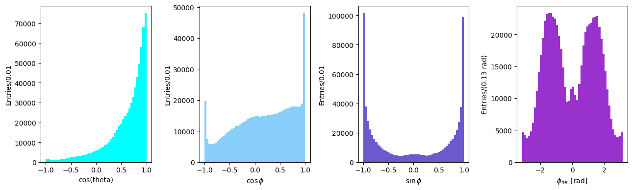
Angular distributions in helicity frame#
Angles and particle directions can be visualised in different reference frames in which resonance properties can emerge more easily. The decay distribution of the dipion may be discussed in the helicity reference system, defined as follows:
The \(z\) direction is chosen opposite to the direction of the recoiling nucleon in the D rest system (i.e., it is equal to the direction of flight of the dipion in the overall c.m. system)
The \(y\) direction is the normal to the production plane, defined by the cross product of the three-momenta of the dipion and the nucleon
The \(x\) direction follows as \(\mathbf{x = y \times z}\).
The decay angles \(\phi,\; \theta\) are defined as the polar and azimuthal angles of the unit vector \(\mathbf n\). In the present case (of a two-particle decay), it indicates the direction of flight of one of the two decay particles; for a three-particle decay, \(\mathbf n\) is the normal to the decay plane in the decaying particle rest frame. The angles are defines as follows:
\(\cos\theta = \mathbf{n\cdot z}\)
\(\cos\phi = \frac{\mathbf{y\cdot(z\times n)}}{|\mathbf{z\times n}|}\)
\(\sin\phi = -\frac{\mathbf{x\cdot(z\times n)}} {|\mathbf{z\times n}|}\)
Let’s choose the \(\pi^+\)’s direction as \(\mathbf n\) and extract the angular distributions for the reaction under study:
n = pip_cm[1:] / pip_cm.p
z = q[1:] / q.p
y = np.cross(k[1:], q[1:], axis=0)
y /= np.linalg.norm(y, axis=0)
x = np.cross(y, z, axis=0)
cos_theta = np.sum(n * z, axis=0)
z_cross_n = np.cross(z, n, axis=0)
cos_phi = np.sum(y * z_cross_n, axis=0) / np.linalg.norm(z_cross_n, axis=0)
sin_phi = -np.sum(x * z_cross_n, axis=0) / np.linalg.norm(z_cross_n, axis=0)
phi_helicity = np.arctan2(sin_phi, cos_phi)
Note on the extraction of the \(\phi\) angle: the angle spans the \((-\pi, +\pi)\) range and its sign is taken correctly into account by the arctan2 function.
Let’s plot the distributions for \(\cos\theta\) and the azimuthal angle \(\phi\) in the helicity frame.
Show code cell source
fig, ax = plt.subplots(1, 4, tight_layout=True, figsize=(13, 4))
ax[0].hist(cos_theta, bins=50, color="aqua")
ax[0].set_xlabel("cos(theta)")
ax[0].set_ylabel("Entries/0.01")
ax[1].hist(cos_phi, color="lightskyblue", bins=50)
ax[1].set_xlabel(R"$\cos\phi$")
ax[1].set_ylabel("Entries/0.01")
ax[2].hist(sin_phi, bins=50, color="slateblue")
ax[2].set_xlabel(R"$\sin\phi$")
ax[2].set_ylabel("Entries/0.01")
ax[3].hist(phi_helicity, bins=50, color="darkorchid")
ax[3].set_xlabel(R"$\phi_\mathrm{hel}$ [rad]")
ax[3].set_ylabel("Entries/(0.13 rad)")
plt.show()
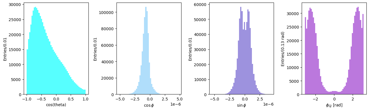
Angular distributions in the Gottfried-Jackson frame#
Differently from the helicity system, in the Gottfried-Jackson system the \(z\) axis is equal to the direction of flight of the incoming photon in the D rest frame. Having replaced the \(z\) axis, all other vectors definitions follow accordingly.
n = pip_cm[1:] / pip_cm.p
z = k_cm_di_pion[1:] / k_cm_di_pion.p
y = np.cross(k[1:], q[1:], axis=0)
y /= np.linalg.norm(y)
x = np.cross(y, z, axis=0)
cos_theta = np.sum(n * z, axis=0)
z_cross_n = np.cross(z, n, axis=0)
cos_phi = np.sum(y * z_cross_n, axis=0) / np.linalg.norm(z_cross_n)
sin_phi = -np.sum(x * z_cross_n, axis=0) / np.linalg.norm(z_cross_n)
phi_GJ = np.arctan2(sin_phi, cos_phi)
Show code cell source
fig, ax = plt.subplots(1, 4, tight_layout=True, figsize=(13, 4))
ax[0].hist(cos_theta, bins=50, color="aqua", alpha=0.66)
ax[0].set_xlabel("cos(theta)")
ax[0].set_ylabel("Entries/0.01")
ax[1].hist(cos_phi, color="lightskyblue", bins=50, alpha=0.66)
ax[1].set_xlabel(R"$\cos\phi$")
ax[1].set_ylabel("Entries/0.01")
ax[2].hist(sin_phi, bins=50, color="slateblue", alpha=0.66)
ax[2].set_xlabel(R"$\sin\phi$")
ax[2].set_ylabel("Entries/0.01")
ax[3].hist(phi_GJ, bins=50, color="darkorchid", alpha=0.66)
ax[3].set_xlabel(R"$\phi_{GJ}$ [rad]")
ax[3].set_ylabel("Entries/(0.13 rad)")
plt.show()
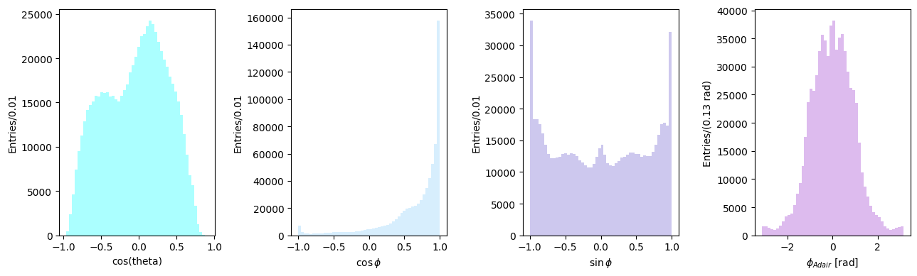
Angular distributions in the Adair frame#
On the other hand, in the Adair system the \(z\) is equal to the direction of flight of the incoming photon in the c.m. system of the reaction. All other definition follow, as above.
n = pip_cm[1:] / pip_cm.p
z = k[1:] / k.p
y = np.cross(k[1:], q[1:], axis=0)
y /= np.linalg.norm(y, axis=0)
x = np.cross(y, z, axis=0)
cos_theta = np.sum(n * z, axis=0)
z_cross_n = np.cross(z, n, axis=0)
cos_phi = np.sum(y * z_cross_n, axis=0) / np.linalg.norm(z_cross_n, axis=0)
sin_phi = -np.sum(x * z_cross_n, axis=0) / np.linalg.norm(z_cross_n, axis=0)
phi_adair = np.arctan2(sin_phi, cos_phi)
Show code cell source
fig, ax = plt.subplots(1, 4, tight_layout=True, figsize=(13, 4))
ax[0].hist(cos_theta, bins=50, color="aqua", alpha=0.33)
ax[0].set_xlabel("cos(theta)")
ax[0].set_ylabel("Entries/0.01")
ax[1].hist(cos_phi, color="lightskyblue", bins=50, alpha=0.33)
ax[1].set_xlabel(R"$\cos\phi$")
ax[1].set_ylabel("Entries/0.01")
ax[2].hist(sin_phi, bins=50, color="slateblue", alpha=0.33)
ax[2].set_xlabel(R"$\sin\phi$")
ax[2].set_ylabel("Entries/0.01")
ax[3].hist(phi_adair, bins=50, color="darkorchid", alpha=0.33)
ax[3].set_xlabel(R"$\phi_{Adair}$ [rad]")
ax[3].set_ylabel("Entries/(0.13 rad)")
plt.show()