Lecture 12 – Relativistic kinematics#
Some exercises on relativistic kinematics using the pylorentz package
Prepare the notebook with the preambles for the inclusion of pandas, numpy and matplotlib.pyplot:
Import Python libraries
import gdown
import matplotlib.pyplot as plt
import numpy as np
import pandas as pd
from pylorentz import Momentum4
output_path = gdown.cached_download(
    url="https://drive.google.com/uc?id=17J4rrO-NHL8whkd7hjELhJbCoanoaqam",
    path="data/antineutron_3pi.dat",
    md5="5ff45076c9d921aa0c9c803b8d2d8958",
    quiet=True,
)
data = pd.read_csv(output_path)
data.columns = data.columns.str.strip()
data
/opt/hostedtoolcache/Python/3.10.14/x64/lib/python3.10/site-packages/gdown/cached_download.py:102: FutureWarning: md5 is deprecated in favor of hash. Please use hash='md5:xxx...' instead.
  warnings.warn(
| p1x | p1y | p1z | E1 | p2x | p2y | p2z | E2 | p3x | p3y | p3z | E3 | pnbar | ||
|---|---|---|---|---|---|---|---|---|---|---|---|---|---|---|
| 0 | -0.649042 | -0.462925 | 0.057760 | 0.811400 | 0.467449 | -0.076535 | 0.248084 | 0.552622 | 0.184921 | 0.542265 | 0.101577 | 0.598368 | 0.407442 | |
| 1 | 0.202017 | -0.331041 | -0.180710 | 0.450038 | 0.472889 | 0.469358 | 0.289029 | 0.739553 | -0.684486 | -0.139534 | 0.282087 | 0.766187 | 0.390522 | |
| 2 | 0.131898 | -0.111253 | 0.063348 | 0.230795 | 0.587119 | 0.420368 | 0.409048 | 0.841556 | -0.715388 | -0.309328 | -0.252149 | 0.830976 | 0.220276 | |
| 3 | 0.338881 | -0.809633 | 0.106584 | 0.895090 | 0.088779 | 0.166919 | 0.040559 | 0.238469 | -0.418469 | 0.641379 | 0.173450 | 0.797526 | 0.320725 | |
| 4 | -0.442309 | 0.269700 | 0.121178 | 0.550035 | 0.858318 | -0.264391 | 0.039060 | 0.909735 | -0.420124 | -0.010746 | 0.112709 | 0.456948 | 0.273031 | |
| ... | ... | ... | ... | ... | ... | ... | ... | ... | ... | ... | ... | ... | ... | ... |
| 11892 | 0.308922 | 0.169041 | -0.057350 | 0.383113 | 0.462751 | 0.186437 | -0.147222 | 0.538564 | -0.770108 | -0.359349 | 0.528571 | 1.010480 | 0.324021 | |
| 11893 | -0.624261 | -0.420438 | 0.023650 | 0.765839 | 0.431008 | 0.650052 | 0.211829 | 0.820175 | 0.202220 | -0.229407 | 0.138572 | 0.363596 | 0.374157 | |
| 11894 | 0.555306 | -0.587870 | 0.101743 | 0.826914 | -0.286882 | -0.089814 | 0.110253 | 0.349289 | -0.276060 | 0.681550 | 0.116628 | 0.757496 | 0.328734 | |
| 11895 | -0.380387 | 0.239558 | -0.333601 | 0.576932 | -0.166609 | -0.491912 | 0.067187 | 0.541968 | 0.547973 | 0.251906 | 0.478946 | 0.782687 | 0.212532 | |
| 11896 | 0.183408 | -0.524653 | -0.293374 | 0.643775 | 0.327122 | 0.363945 | 0.123429 | 0.523620 | -0.509498 | 0.151911 | 0.570773 | 0.792418 | 0.400922 |
11897 rows × 14 columns
The columns headers present some trailing blanks, that must be dropped to be able to use correctly the DataFormat structure (if not, they deliver an error message). To do so, the
str.strip()method must be used beforehand to reformat the column shape.
The file contains the 4-momenta of the particles of the reaction \(\bar n p \rightarrow \pi^+_1\pi^+_2\pi^-_3\), the last column corresponds to the 3rd component of the antineutron momentum (up to 300 MeV/c), which travels along the \(z\) axis
Load the pylorentz package (if not available, install it with pip install pylorentz). Let’s import the arrays from the csv table into Momentum4 objects and repeat the calculation of invariant masses and other observables. We are working with numpy arrays whose length is equale to the number of entries of the table read from the csv file.
# final state
pi1 = Momentum4(data.E1, data.p1x, data.p1y, data.p1z)
pi2 = Momentum4(data.E2, data.p2x, data.p2y, data.p2z)
pi3 = Momentum4(data.E3, data.p3x, data.p3y, data.p3z)

# initial state
m_neutron = 0.93956
m_proton = 0.93827
n_events = len(data)
zeros = np.zeros(n_events)
ones = np.ones(n_events)
E_nbar = np.sqrt(m_neutron**2 + data.pnbar**2)
nbar = Momentum4(E_nbar, zeros, zeros, data.pnbar)
target = Momentum4(m_proton * ones, zeros, zeros, zeros)
system12 = pi1 + pi2
system23 = pi2 + pi3
system13 = pi1 + pi3

invariantMassSquared12 = system12.m2
invariantMassSquared13 = system13.m2
invariantMassSquared23 = system23.m2
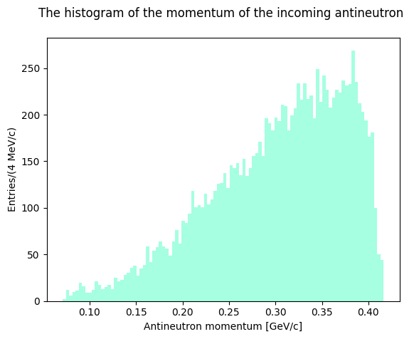
Let’s plot the Dalitz Plots using the new Momentum4 objects. As in the first exercise let’s plot the antineutron momentum to see how the distribution looks like.
plt.hist(nbar.p, bins=100, color="aquamarine", alpha=0.7)
plt.xlabel("Antineutron momentum [GeV/c]")
plt.ylabel("Entries/(4 MeV/c)")
plt.title("The histogram of the momentum of the incoming antineutron \n")
plt.show()
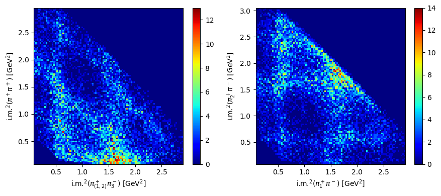
And now let’s plot the two Dalitz plots with the square invariant masses of the pion pairs:
Show code cell source
fig, ax = plt.subplots(1, 2, tight_layout=True, figsize=(9, 4))
h0 = ax[0].hist2d(
    invariantMassSquared13, invariantMassSquared12, bins=100, cmap="jet"
)
h0 = ax[0].hist2d(
    invariantMassSquared23, invariantMassSquared12, bins=100, cmap="jet"
)
fig.colorbar(h0[3], ax=ax[0])
ax[0].set_xlabel(R"i.m.$^2(\pi^+_{(1,2)}\pi^-_{3}$) [GeV$^2$]")
ax[0].set_ylabel(R"i.m.$^2(\pi^+\pi^+$) [GeV$^2$]")
h1 = ax[1].hist2d(
    invariantMassSquared13, invariantMassSquared23, bins=100, cmap="jet"
)
h1 = ax[1].hist2d(
    invariantMassSquared23, invariantMassSquared13, bins=100, cmap="jet"
)
fig.colorbar(h1[3], ax=ax[1])
ax[1].set_xlabel(R"i.m.$^2(\pi^+_1\pi^-$) [GeV$^2$]")
ax[1].set_ylabel(R"i.m.$^2(\pi^+_2\pi^-$) [GeV$^2$]")
plt.show()
Let’s transform the 4-momenta of the particles, which are defined in the lab system, into the center-of-mass system exploiting the boostparticle function of pylorentz:
cm = nbar + target
pi1_cm = pi1.boost_particle(-cm)
pi2_cm = pi2.boost_particle(-cm)
pi3_cm = pi3.boost_particle(-cm)
nbar_cm = nbar.boost_particle(-cm)
target_cm = target.boost_particle(-cm)
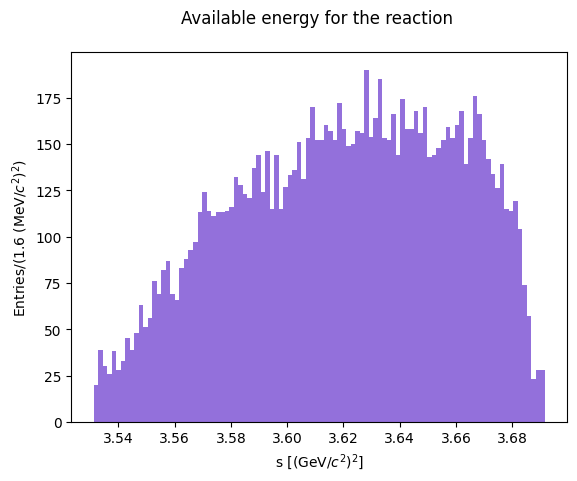
Let’s check whether the Mandelstam variables are indeed invariant in the different reference systems. Let’s assume a two-body reaction \(a + b\rightarrow c + d\) where in the final state two pions form a neutral dipion which recoils against the remaining \(\pi^+_2\): \(\bar n + p \rightarrow D(\pi^+_1\pi^-_3) + \pi^+_2\)
total energy \(s = (p_a+p_b)^2 = (p_c + p_d)^2\)
s_lab = cm.m2
print(s_lab)
[3.68488927 3.67247922 3.57405227 ... 3.63104835 3.57079063 3.68005438]
initCM = nbar_cm + target_cm
s_cm = initCM.m2
print(s_cm)

s_lab - s_cm
[3.68488927 3.67247922 3.57405227 ... 3.63104835 3.57079063 3.68005438]
array([ 4.4408921e-16,  8.8817842e-16, -8.8817842e-16, ...,
       -4.4408921e-16,  0.0000000e+00,  4.4408921e-16])
Show code cell source
plt.hist(s_lab, bins=100, color="MediumPurple")
plt.xlabel("s [(GeV/$c^2)^2$]")
plt.ylabel("Entries/(1.6 (MeV/$c^2)^2$)")
plt.title("Available energy for the reaction \n")
plt.show()
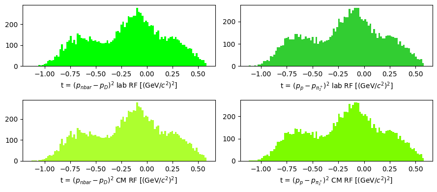
Momentum transfer \(t = (p_a - p_c)^2 = (p_b - p_d)^2\)
dipion = system13
t_lab_1 = (nbar - dipion).m2
t_lab_2 = (target - pi2).m2
dipion_cm = system13.boost_particle(-cm)
t_cm_1 = (nbar_cm - dipion_cm).m2
t_cm_2 = (target_cm - pi2_cm).m2
Show code cell source
fig, ax = plt.subplots(2, 2, tight_layout=True, figsize=(9, 4))
ax[0, 0].hist(t_lab_1, bins=100, color="Lime")
ax[0, 0].set_xlabel(R"t = $(p_{nbar} - p_D)^2$ lab RF [$(\mathrm{GeV}/c^2)^2$]")
ax[0, 1].hist(t_lab_2, bins=100, color="LimeGreen")
ax[0, 1].set_xlabel(R"t = $(p_p - p_{\pi^+_2})^2$ lab RF [$(\mathrm{GeV}/c^2)^2$]")
ax[1, 0].hist(t_cm_1, bins=100, color="GreenYellow")
ax[1, 0].set_xlabel(R"t = $(p_{nbar} - p_D)^2$ CM RF [$(\mathrm{GeV}/c^2)^2$]")
ax[1, 1].hist(t_cm_2, bins=100, color="LawnGreen")
ax[1, 1].set_xlabel(R"t = $(p_p - p_{\pi^+_2})^2$ CM RF [$(\mathrm{GeV}/c^2)^2$]")
plt.show()
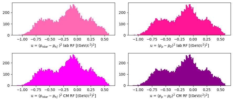
\(u = (p_a - p_d)^2 = (p_b - p_c)^2\)
u_lab_1 = (nbar - pi2).m2
u_lab_2 = (target - dipion).m2
u_cm_1 = (nbar_cm - pi2_cm).m2
u_cm_2 = (target_cm - dipion_cm).m2
Show code cell source
fig, ax = plt.subplots(2, 2, tight_layout=True, figsize=(9, 4))
ax[0, 0].hist(u_lab_1, bins=100, color="HotPink")
ax[0, 0].set_xlabel(
    R"u = $(p_{nbar} - p_{\pi^+_2})^2$ lab RF [$(\mathrm{GeV}/c^2)^2$]"
)
ax[0, 1].hist(u_lab_2, bins=100, color="DeepPink")
ax[0, 1].set_xlabel(R"u = $(p_p - p_D)^2$ lab RF [$(\mathrm{GeV}/c^2)^2$]")
ax[1, 0].hist(u_cm_1, bins=100, color="Fuchsia")
ax[1, 0].set_xlabel(
    R"u = $(p_{nbar} - p_{\pi^+_2})^2$ CM RF [$(\mathrm{GeV}/c^2)^2$]"
)
ax[1, 1].hist(u_cm_2, bins=100, color="DarkMagenta")
ax[1, 1].set_xlabel(R"u = $(p_p - p_D)^2$ CM RF [$(\mathrm{GeV}/c^2)^2$]")
plt.show()
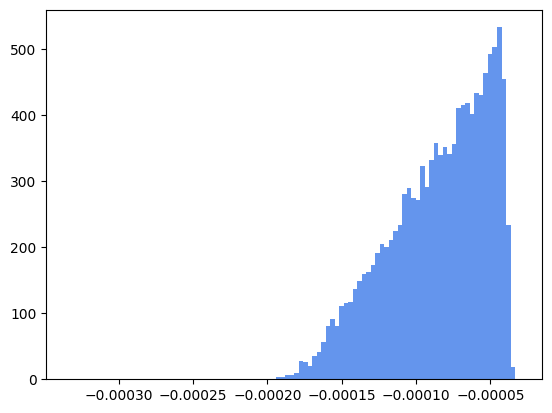
Test if \(\; s + t + u = m_1^2 + m_2^2 + m_3^2 + m_4^2\)
mandelstam_sum = s_lab + t_lab_1 + u_lab_1
m2_sum = m_neutron**2 + m_proton**2 + dipion_cm.m2 + pi2_cm.m2
Show code cell source
plt.hist(mandelstam_sum - m2_sum, bins=100, color="CornFlowerBlue")
plt.show()
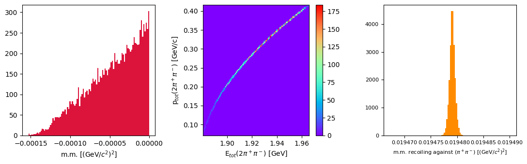
Another interesting quantity to be observed is the missing mass. It can be evaluated comparing the total energies between the initial and the final state of a reaction, or, given a final state, evaluating the missing energy recoiling against a system of particles. In any case, the missing mass quantity is defined as the modulus of the 4-momentum corresponing to the difference of the 4-momenta of the involved particles.
# missing mass between initial and final state
p4_initial_state = cm
p4_final_state = pi1 + pi2 + pi3
p4_missing = p4_initial_state - p4_final_state
# missing mass recoiling against the neutral dipion systems (there are two)
dipion1 = pi1 + pi3
dipion2 = pi2 + pi3
recoiling_missing_mass1 = p4_final_state - dipion1
recoiling_missing_mass2 = p4_final_state - dipion2
Let’s plot the missing mass of the reaction, the scatter plot of total momentum versus total energy of the measured particles in the final state (it should be close to zero), and the missing mass recoiling against the neutral dipion (it should be close to the mass of a pion, for a correctly selected exclusive reaction).
Show code cell source
fig, ax = plt.subplots(1, 3, tight_layout=True, figsize=(11, 3.5))
ax[0].hist(p4_missing.m2, bins=100, color="crimson")
ax[0].set_xlabel(R"m.m. [$(\mathrm{GeV}/c^2)^2$]")
# ptot vs Etot plot
h1 = ax[1].hist2d(p4_final_state.e, p4_final_state.p, bins=100, cmap="rainbow")
fig.colorbar(h1[3], ax=ax[1])
ax[1].set_xlabel(R"$\mathrm{E}_{tot}(2\pi^+\pi^-)$ [GeV]")
ax[1].set_ylabel(R"$\mathrm{p}_{tot}(2\pi^+\pi^-)$ [GeV/c]")
# missing mass recoiling against the neutral dipion (2 entries/event)
all_missing_dipion = np.concatenate(
    [recoiling_missing_mass1.m2, recoiling_missing_mass2.m2]
)
missingHisto = ax[2].hist(all_missing_dipion, bins=100, color="darkorange")
ax[2].set_xlabel(R"m.m. recoiling against $(\pi^+\pi^-)$ [$(\mathrm{GeV}/c^2)^2$]")
ax[2].xaxis.get_label().set_fontsize(8)
ax[2].tick_params(axis="both", which="major", labelsize=8)
plt.show()
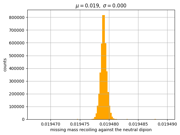
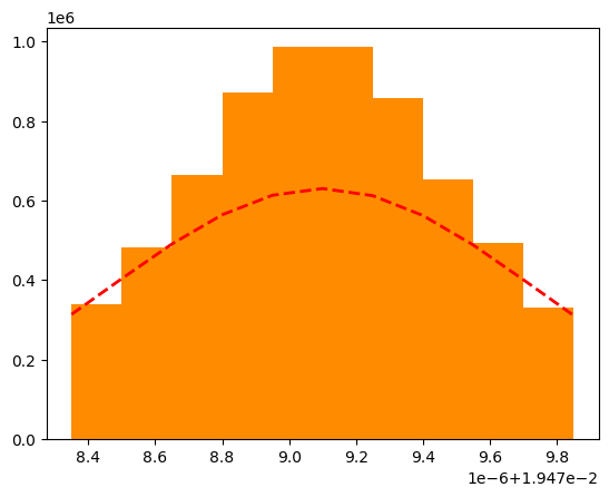
Let’s fit the last plot with a gaussian function to check if the missing particle is really a charged pion (mass: 0.140 GeV/\(c^2\)).
from scipy.stats import norm

# best fit of data
mu, sigma = norm.fit(all_missing_dipion)

# the histogram of the data
n, bins, patches = plt.hist(
    all_missing_dipion,
    range=(0.01947835, 0.01947985),
    density=True,
    facecolor="darkorange",
    histtype="barstacked",
)

# add a 'best fit' line
y = norm.pdf(bins, mu, sigma)
l = plt.plot(bins, y, "r--", linewidth=2)
print("The missing mass in GeV/c^2 is: ", np.sqrt(mu))
The missing mass in GeV/c^2 is: 0.13956753832275667
Show code cell source
plt.xlabel("missing mass recoiling against the neutral dipion")
plt.ylabel("counts")
plt.title(Rf"$\mu={mu:.3f},\ \sigma={sigma:.3f}$")
plt.grid(True)
plt.hist(
    all_missing_dipion, 100, density=True, facecolor="orange", histtype="barstacked"
)
plt.show()